Unsupervised Segmentation Method of Multicomponent Images based on Fuzzy Connectivity Analysis in the Multidimensional Histograms ()
1. Introduction
In many fields such as medicine, food, robotics, security systems, etc, the acquisition and the analysis of images are essential processes for taking decisions [1-4], as it is often difficult to perform them manually, it is necessary to automate certain tasks by computing. Thus in this paper, we present, a new vectorial segmentation method based more particularly on the full n-D compact histograms by a fuzzy connexity analysis.
Segmentation is an important step in image processing and automatic pattern recognition proces-ses based on image analysis as subsequent extracted data are highly dependent on the accuracy of this operation. In general, the automated segmentation is one of the most difficult tasks in image analysis [5], because a false segmentation will cause degradation of the measurement process and therefore the interpretation may fail. The segmentation methods based on the analysis of color histograms are facing the difficulty of treating a huge quantity of information: for a color image of resolution N ´ M with each component coded on 8 bits, a classical 3D histogram is an array of 224 cells, the number in each cell being coded on at least log2(MN) bits in order to store the number of pixels of each color allowed. In the case where M = N = 256, the standard 3-D histogram requires 128 Mo.
A few years ago, we have proposed a new way of coding the nD histograms, leading to the so-called compact histogram [6], in which only the occupied cells of the classical histogram are memorised. This reduces the memory space required drastically: it is lowered to a value of 500 ko for a 256 ´ 256 image with color components coded on 8 bits, without any loss of color information, it shows its efficiency in previous articles [7,8].
Using histograms for classifying colour pixels can be achieved through four different strategies.
The first strategy proceeds in a marginal way. Each component of the histogram is examined separately [9,10]. The method is easy to implement, but it does not take into account the correlation between colorimetric components.
In the second strategy, each colorimetric component is requantized on q bits (q < 8) in order to reduce the histogram size [11]. The method is efficient, but it makes an a priori color classification.
The third strategy that many authors have developed proceeds by projection of the 3-D histogram on two of the three colorimetric axes. We have developped this strategy in a previous paper [12] and used also in other articles such as [13-15]; The histogram, with populations requantized on 256 levels, is considered as a gray level image and processed by a watershed algorithm. The correlation between components is partially taken into account, but the requantization of the populations alters the true histogram, and the projection can result in ignoring some significant classes.
Here we propose a fourth strategy. It is fully vectorial, which is allowed by the use of the compact n-D histogram. Its principle consists in finding the peaks of classic multidimensional histogram using the compact multidimensional histogram by the consideration of a model of fuzzy neighbourhood. The kernels of the built classes correspond to the peaks retained using the algorithm for labelling connected components with binary fuzzy neighbourhood that we realized in this work, it accepts two input parameters which are the degree of fuzzy connectedness expressing the similarity between the vector points of the compact n-D histogram and a population threshold limiting the class size. The choice of the fuzzy connectedness here is justified by the difficulty of defining a net similarity between the vector points attribute or “colors” of the pixels of the image [16,17]. This leads to different results of segmentation of the same number of classes for different values of pairs of thresholds. Assessing the quality of segmentation can choose the most relevant segmentation. The results of our multidimensional segmentation method are compared to those of the method of classification K-means [13,18, 19] in order to evidence the performance of our approach using supervised and unsupervised [20-23] evaluation methods of the segmentation quality.
2. A Fast and Compact Multidimensional Histogram
We consider multicomponent images (for example multispectral images) with n components , for i = 1 to n, each Ii has a tonal resolution of Q possible values and each pixel of spatial coordinate
  takes a value among the Q possibilities. A n-dimensional histogram of such an image would comprise Qn cells. For an image with N pixels of resolution, only at most N of these Qn cells can be occupied, meaning, as n grows, most of the cells of the n-dimensional histogram are in fact empty. For example, for a commun 512 × 512 RGB color image with n = 3 and Q = 256, there are Qn = 2563 ≈ 16 × 106 colorimetric cells of n-tuples with at most only 3N = 5122 = 262144 of them which can be occupied. The idea of a compact representation of the n-dimensional histogram [6], where only those cells that are occupied are coded. The n-dimensional histogram is coded as a linear array where the entries are the n-tuples (the colors) present in the image and arranged in lexicographic order of their components (I1, I2,
  , In). To each entry (in number ≤ N) is associated the number of pixels in the image having this n-value (this color). An example of this compact representation of the n-dimensional histogram is shown in Table 1.
The practical calculation of such a compact histogram starts with the lexicographic ordering of the N n-tuples corresponding to the N pixels of the image. The result is a linear array of the N ordered n-tuples with their population. With a dichotomic quick sort algorithm to realize the lexicographic ordering, the whole process of calculating the compact multidimensional histogram can be achieved with an average complexity of O(N logN), independent of the dimension n. Therefore, both compact
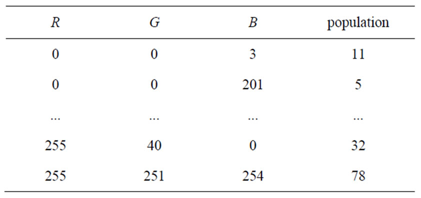
Table 1. An example of compact coding of the 3-dimensional histogram of an RGB color image with Q = 256. The entries of the linear array are the components (I1, I2, I3) = (R, G, B) arranged in lexicographic order, for each color present in the image, and associated to the population of pixels having this color.
representation and its fast calculation are afforded by the process for the multidimensional histogram. For example, for a 9-component 838 × 762 satellite image with Q = 256, the compact histogram was calculated in about 5 s on a standard 1 GHz clock desktop computer, with a coding volume of 1.89 Moctets, while the classic histogram would take 3.60 × 10¹⁶ Moctets completely unmanageable by today’s computers.
The advantages of the compact multidimensional applied to multicomponent images (see Figure 1) are shown in Table 2.
3. Fuzzy Connected Components Labeling of Compact Histogram
3.1. Formalism of Fuzzy Logic and Concept of Fuzzy Neighbourhood
We present here some aspects of the theory of fuzzy logic, fundamental to understanding the algorithm of Fuzzy Connected Component Labeling (FCCL) compact multidimensional histograms, developed in following sections. The reader will find a complete overview in [24].
X denote the universe of reference, consisting of elements x, and place us first in the theory of classical ensembles, that is to say net. Then any subset A of X net is completely defined by its characteristic function µAdefined on the set {0,1} score, by:
 (1)
(1)
If the set score is now the continuum [0,1], A becomes a fuzzy subset of X, and µA is its membership function. The subset A is then defined by:
 (2)
(2)
An α-cut of A is the net subset of items with a membership degree to A greater than or equal to α. It is noted Cα(A):
 (3)
(3)
The concept of fuzzy relation is a generalization with the fuzzy domain of the concept of equivalence relation defined in the net case. A fuzzy relation can be measured by a scalar in the interval [0,1], the degree to which a logical proposal is verified. With a fuzzy relation R is associated membership function, denoted by µR. Let X and Y be two universes of reference, the respective elements x and y. A fuzzy relation between the elements of these two worlds is formally defined as:
 (4)
(4)

Figure 1. Example of multicomponent images.
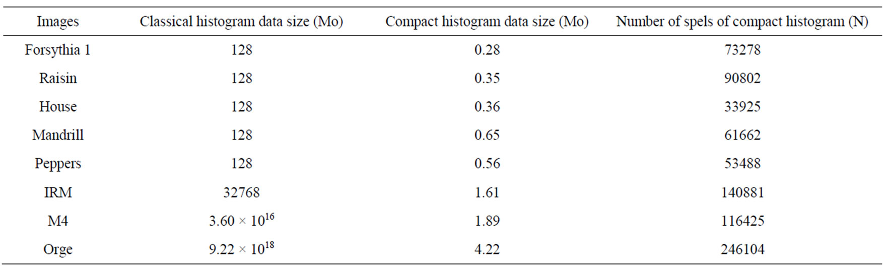
Table 2. Comparative table of volumes of the classical and compact histograms of the images of Figure 1.
When X=Y, the fuzzy relation is known as binary.
In one of the following sections will be built a fuzzy connected component labeling of compact multidimensional histogram (it is him which plays the role of universe of reference X). The labelling will use a binary fuzzy relation, which we call fuzzy similarity, assessing the degree of similarity between two spells x and y of compact histogram multidimensional. The membership function of this relationship will be expressed as:
 (5)
(5)
This model of fuzzy neighborhood is used in many studies [25,26]. In our case, the threshold M is set at 7 which is the maximum distance allowed so that two spells resembles itself, and the distance d considered will be that of Chebychev or again call Queen-wise distance, given by the following equation:
 (6)
(6)
3.2. Classical Connected Components Labelling
We have recently achieved [8] the connected components labelling (CCL) of n-D compact histograms. It consists in sweeping all the n-tuples present in the compact histogram, in order to gather, under the same label, the n-uplets which are neighboring in the n-D colorimetric space.
Since the n-uplets are ordered in lexicographical order inside the compact histogram, labelling a n-tuple is achieved by sweeping only the (3n − 1)/2 n-tuples connected neighbours preceding it. For example, Table 3 shows the four doublets of (i,j) to be swept for labelling the doublet (i,j) in the case of 2-D compact histograms.
The CCL is applied to the full n-D compact histograms of five multicomponent images (see Figure 1)

Table 3. Connected neighbours to be swept for CCL of doublet (i, j) in the case of a 2-D compact histogram (colorimetric axes I and J).
taken on the web site of gdr-isis. Table 4 shows the number of connected components (CC) of their histograms and, the minimum and maximum size of CC are expressed as number of pixels compared to the size of the images.
3.3. Principle of Fuzzy Connected Components Labelling
The connected component labeling with fuzzy neighborhood (CCLF) is based on the notion of fuzzy connectedness and requires the definition of a fuzzy similarity relation between the spells. Contrary to the notion of net neighborhood, a fuzzy neighborhood is defined on a fuzzy subset. In the literature, several studies take into account the spatial information in the definition of fuzzy similarity relation [27,28]. Our neighborhood fuzzy model disregards the fact that we work solely on the histogram. The model of neighborhood fuzzy (fuzzy similarity) selected is defined by Equation (5). The cost of a path between two related spells c and d in the histogram
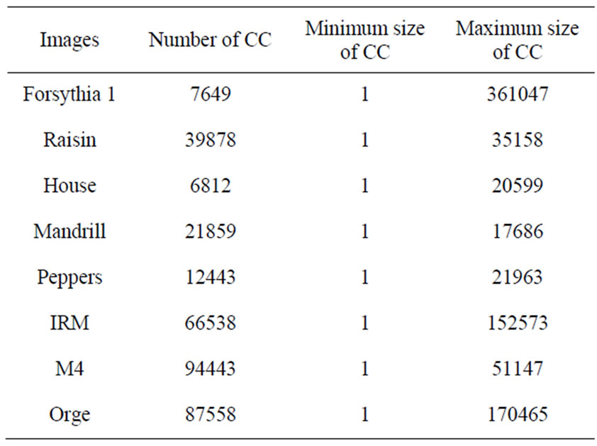
Table 4. Statistics in related connected components of the images of Figure 1.
can be defined by the fuzzy relation  as:
as:
 (7)
(7)
où is a path between the spells C1 = c and Cm = d. As several paths may exist between spell c and d, the overall cost of the paths is defined as the maximum value of all path costs calculated on the set of paths. The overall cost of paths between two related spell c and d in the histogram can then be defined by the fuzzy relation
  as:
as:
 (8)
(8)
The fuzzy relation  is an equivalence relation. The definition of a
  -neighborhood between two spels requires to fix a minimum threshold of similarity which we denote
 . This threshold being fixed, find the predecessors of a spel c returns searching its neighbors of a minimum cost
  i.e. the spels of the net set
  -cut of the fuzzy relation
 .
.
Let d be an element of the set of predecessors of c in the compact histogram Hc.
 (9)
(9)
The principle of the CCLF is similar to that of the CCL, with for only difference the research of predecessors of a spel in compact histogram as shown by Equation (9). In practice we will vary the value of  to study its influence on the number of connected components. Two values bring back to us to particular cases:
• when , the spels of the compact histogram are considered each one as a connected component, so the number of connected components equals the number of spels;
• when  the CCLF corresponds to the CCL.
3.4. Our Algorithm of Fuzzy Connected Components Labelling
The proposed algorithm integrates the search of fuzzy predecessors, their number being limited by the fixation of overall cost . The algorithm returns as output the vector E containing the labels of spels as they appear in the compact histogram, and the number of connected components (NberCc) of the histogram.

//Hc: compact n-D histogram
//E: table of spels label
//NberCc: number of connected components
//Tequiv: management table of equivalences Label
//taille: function that returns the number of rows in a table
//elimineRedondance: removes redundant elements of an array
//max: function that returns the maximum of an array
//min: function that returns the minimum of a table
N = taille(Hc) //number of spels of n-D compact histogram
E(1) = 1 //label of the first spel of Hc to 1
Tequiv(1) = 1 //equivalence label 1 to 1
For i = 2: N
P = Hc(i,:) //current spel labeling
j = i – 1
IndexPred = Ø

For j =1: i – 1
While ( )
)
c = Hc(j,:)
If ( )
)
IndexPred = [Index-
Pred; j]
EndIf
EndWhile
EndFor
If (taille(IndexPred)  0)
0)
Etiq = E(IndexPred)//returns the labels of the predecessors
Etiq = elimineRedondance(Etiq)
EndIf
If (taille(Etiq) == 0)
E(i) =1 + max(E)
Tequiv(E(i)) = E(i)
ElseIf (taille(Etiq) ==1)
E(i) = Etiq
Else
E(i) = min(Etiq)
Tequiv(E(IndexPred)) = E(i)
EndIf
EndFor
For i = 2:N
E(i) = Tequiv(E(i)) //global update of labels
EndFor
3.5. Example of Results
The FCCL algorithm is applied on the compact n-D histograms of multicomponent images in Figure 1. Table 5 illustrates the results for different values of . It shows that when the degree of similarity
  decrease, the number of connected components (CC) decrease.
4. Fuzzy Vectorial Classification of Tuples
4.1. Principle
The classification of colours is carried out in two steps: the learning step and the decision step.
The learning step is a hierarchical decomposition of populations in the compact n-D histogram. For each level of population pn, peaks Pi are identified by the FCCL algorithm for a given value of α, which retains the connected components whose populations are greater than or equal to pn. Each peak is then iteratively decomposed into narrower peaks, beginning from population 0. A peak is labelled as significant if it represents a population greater than or equal to a threshold S (expressed in percent of the total population in the histogram). The procedure is illustrated in part (a) of Figure 2 (drawn in one dimension for clarity). We shall name kernels Ki the peaks corresponding to circled leaves in part (b) of Figure 2. In other words, kernels are significant peaks (part (a) of Figure 2) without descendants in the hierarchical decomposition tree (part (b) of Figure 2) (e.g., Figure 2 shows five significant peaks Pi (i = 0 to 4) and three kernels Ki (i = 2, 3, 4)). The number of classes Nc is taken equal to the number of kernels (the class corresponding to kernel Ki is noted Ci). Therefore Nc depends

Table 5. Statistics in related fuzzy connected components of the images of Figure 1.
 (a) (b)
Figure 2. An example of hierarchical decomposition with α = 0.5. The circled leaves (part (b)) correspond to significant peaks as obtained at the end of the iterative decomposition (solid lines in part (a)), whereas leaves marked < S (part (b)) correspond to insignificant peaks (dotted lines in part (a)).
on the threshold S, i.e. on the precision the image colors are analyzed with and the value of α the degree of similarity between the spels.
In the decision step, the mass center µ(Ki) of each kernel Ki is calculated in the feature multidi-mensional space. Let us denote by ß the color corresponding to the point of coordinates (g1, g2,  , gn) in the feature space. Two cases appear: if (g1, g2,
  , gn) belongs to Ki, color ß is attributed to class Ci; if not, let us denote by Pk the peak which belong to (g1, g2,
  , gn); color ß is attributed to class Ci corresponding to kernel Ki, son of Pk, such that d[µ(Ki), (g1, g2,
  , gn)] is minimum, where d[y, z] is the Euclidean distance between y and z.
We give a name of this method that we call HierarchieFuzzy_nD.
4.2. Results of Segmentation
The following figure denote Figure 3 shows an example of segmented images by Hierarchie-Fuzzy_nD and K-means methods.
5. Methods for Assessing the Quality of Segmentation
Image segmentation is a fundamental process in image and video analysis. Several approaches have been put forward in the literature [22,29]. We have the region, contour and texture approaches, but this work interests the region approach. It is often used to partition an image into separate regions, which ideally correspond to different

Figure 3. Example of segmented images by HierarchieFuzzy_nD and K-means methods.
real-world objects.
Many segmentation methods exist in literature, but it is difficult to evaluate the efficiency and to make an objective comparison of different segmentation methods. This general problem has been addressed for the evaluation of a segmentation result [20]. There are two main approaches:
• There are supervised evaluation criteria based on the computation of a dissimilarity measure between a segmentation result and ground truth. Baddeley’s distance [30], Vinet’s measure [31], or Hausdorff’s measure [32] are examples of supervised evaluation criteria. In practice the ground truth of natural images is a segmentation results manually made by experts.
• There are unsupervised evaluation criteria that enable the quantification of the quality of a segmentation result without any a priori knowledge. These criteria generally compute statistical measures such as standard deviation or the disparity of each region or class in the segmentation result [33-36].
Currently in practice, no evaluation criterion appears to be satisfactory in all cases [22]. However, we choose here the best criterion for each type of evaluation, i.e. Vinet measure for supervised evaluation and Zeboudj measure in unsupervised case [22].
One potential benefit of supervised methods over unsupervised methods is that the direct comparison between a segmented image and a reference image is believed to provide a finer resolution of evaluation, and as such, discrepancy methods are commonly used for objective evaluation. However, manually generating a reference image is a difficult, subjective, and time-consuming task [20].
5.1. Vinet Measure
The Vinet’s measure [31] that is a supervised criterion which corresponds to the correct classification rate is used as reference for the analysis of the synthetic images. In this case, the ground truth is available. This criterion is often used to compare a segmentation result  with a ground truth
  in the literature. We compute the following superposition table:
 (10)
(10)
Where  is the number of pixels resulting from the intersection of regions
  and
and  in the ground truth. The best match between
  and
and  is one that maximizes
 . Vinet’s measure gives a dissimilarity measure, it is computed as follows:
 (11)
(11)
This criterion is often used to compute correct classification rate of the segmentation result of a synthetic image.
5.2. Zeboudj Criterion
Zeboudj [35] proposed a measure based on the combined principles of maximum interregions disparity and minimal intraregion disparity measured on a pixel neighborhood. Zeboudj’s criterion is defined by:
 (12)
(12)
Where  is the disparity of the region
 .
.
This criterion is suitable for evaluating segmentation of homogeneous and little texture images.
6. Results and Discussion
The tests were performed on many multicomponent images. A synthetic illustration of the evaluation of our method of segmentation is applied to images of Figure 1 with a variation in the number of classes per image to be segmented.
Indexed Tables 6(a) to (e) contains the results of the unsupervised evaluation applied to different images of which we doesn’t ground-truth. However Table 7 illustrates the results of the supervised evaluation obtained from 24 images of forsythia and 1 grape image of which we have their ground-truth.
The relevance of our method of segmentation is made with respect to k-means known in the world of image processing because of its simplicity and its performance.
The Table 7 shows that in supervised evaluation, the fuzzy multidimensional hierarchical method of segmentation HierarchieFuzzy_nD outperforms k-means for each image. This is explained by its ability to detect colorimetrically or spectrally similar classes.
The indexed Table 6 by (a) to (e) evaluates in a synthetic way HierarchieFuzzy_nD comparing it systematiccally to k-means and by putting forward the evaluation of HierarchieFuzzy_nD in the case of the classical connexity between spels i.e. for α = 0,5. Thus can be drawn the following conclusions:
• The segmentation method HierarchieFuzzy_nD proposed gives better results overall compared to k-means as well for color images as multicomponent images in unsupervised evaluation. This is justified by taking into account the uncertainty in the spectral data by solving the problem of colorimetric or spectral similarity between spels of the multidimensional histogram.
• While limiting oneself to alpha = 0,5 corresponding to the traditional connexity, we note that for the images M4 and Orge of which the number of spectral plans is high, that HierarchieFuzzy_nD is systematically considered to be less powerful than k-means. This lower performance is a consequence of the phenomenon of over-segmentation justified by the Table 4 which shows the widespread problem of the spels of the nD histograms in a multidimensional space when n is large, hence the interest of the introduction of fuzzy connectedness between spels characterized by the parameter α, highlighting the relevance of HierarchieFuzzy_nD. The major drawback of this last is to be costly in computing time.

Table 7. Supervised evaluation of real images segmentation; in red, segm-entations considered to be the best.
7. Conclusion
This work is a contribution to the classification by the analysis of multidimensional histograms. It proposes a vectorial strategy to segment color or multicomponent images and provides the tools necessary for its implementation. This work is accompanied by a more general reflexion on the principle of classification in a multidimensional space in connection with the evaluation methods of segmentation.
We have liberated the large volume of multidimensional histograms using the nD compact histogram for which we have proposed a fuzzy algorithm for labeling connected components. This algorithm allowed us to develop an unsupervised and nonparametric method by vectorial classification of multidimensional histograms. We made a solution to the problem of over-segmentation generated by the appearance diffuse of multidimensional histograms and evaluated our segmentation results.
We chose to approach the Classification by analyzing histograms nonparametrically with emphasis on algorithmic and geometric approaches comparatively to statistical approaches. We justify this choice by the need first there was to provide solutions to the problem of dealing vectorially histograms of multicomponent images because of their size. The tools that we have developed, allowed us to better understand the mechanism of classification in a multidimensional space and to open channels to predict outcomes.
In perspective, this work can be directly exploited to define new vectorial methods or strategies for the analysis of multidimensional histograms and their classification. The algorithms developed here can be used to serve statistical or spatio-colorimetric approaches for the segmentation of color and multicomponent images.