1. Introduction
Numerical analysis is the study of set of rules that use numerical estimation for the problems of mathematical analysis as distinguished from discrete mathematics. Fractional differential equations are operational and most effective tool to describe different physical phenomena such as rheology, diffusion processes, damping laws, and so on. Many technics have been delegated to solve differential equation of fractional order. Different structures are used to resolve the issues of nonlinear physical models of fractional orders like Finite element method [1] , Finite difference method [2] , differential transformation method [3] [4] , Adomian’s decomposition method [5] [6] [7] , variational iteration method [8] [9] [10] , Homotopy perturbation technique [11] , Zubair decomposition method (ZDM) [12] , (G’/G)-expansion method [13] , (U’/U)-expansion method [14] , U- expansion method [15] , Fractional sub numerical announcement method [16] [17] , Legendre wavelets technique [18] , Chebyshev wavelets framework [19] [20] [21] , Haar wavelets schema [22] , Legendre Method [23] , Chebyshev strategy [24] , Jacobi polynomial scheme [25] and collocation scheme [26] [27] [28] [29] . All the mentioned approaches have certain limitations like excessive computational work, less efficiency to tackle nonlinearity and divergent solution due to which many issues arise. All these disputes can be fixed with the help of orthogonal polynomials, which is a vital thought in close estimation and structures. These orthogonal polynomials are the reason of powerful strategies of spectral methods [30] [31] [32] . Starting late, Khader [33] displayed a capable numerical procedure for enlightening the fractional order physical problems using the Chebyshev polynomials. In the [34] two Chebyshev spectral frameworks for measuring multi-term fractional problems are displayed. The author (Tamour Zubair) devolve a new wavelets algorithm to construct the numerical solution of nonlinear Bagley-Torvik equation of fractional order which will have less computational works, straight forward and better accuracy as compare to the existing technique. It is to be emphasized that proposed algorithm is tremendously simple but highly effective Moreover, this new pattern is proficient for reducing the computational work to a tangible level while still retaining a very high level of accuracy.
2. Basic Definitions
Fractional Calculus [35] - [40]
We give some basic definitions and properties of the fractional calculus theory which are used further in this paper.
Definition 1. A real function  is said to be in the space
  if there exists a real number
 , such that
 , where
  , and it is said to be in the space
  iff
iff .
.
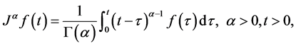
Definition 2. The Riemann-Liouville fractional integral operator of order , of a function
  is defined as

Properties of the operator  can be found in literature, we mention only the following: For
  and
and :
:
1) 
2) 
3) 
The Riemann-Liouville derivative has certain drawbacks when trying to model real-world processes with fractional differential equations. Therefore, we shall introduce a improved fractional differential operator  proposed by
![]() .
.
Definition 3. The fractional derivative of ![]() in the Caputo sense is defined as
in the Caputo sense is defined as
![]()
for![]() . For the Caputo’s derivative we have
. For the Caputo’s derivative we have ![]()
![]() is a constant,
is a constant,
![]()
We use the ceiling function ![]() to denote the smallest integer greater than or equal to
to denote the smallest integer greater than or equal to![]() , and
, and![]() . Recall that for
. Recall that for![]() , the Caputo differential operator coincides with the usual differential operator of integer order.
, the Caputo differential operator coincides with the usual differential operator of integer order.
3. Bagley-Torvik Equations
Bagley-Torvik equation assumes an extremely vital part to study the performance of different material by application of fractional calculus [40] [41] . It has increased its significance in many fields of industrial and applied sciences. Precisely, the equation with 1/2 order derivative or 3/2 order derivative can be model the frequency dependent damping materials. The summed up form of Bagley-Torvik equation is given
![]() (1)
(1)
with initial condition
![]()
with boundary condition at![]() , for
, for![]() , is given by
, is given by
![]()
where ![]() is the nonlinear operator of the equation,
is the nonlinear operator of the equation, ![]() is unknown function.
is unknown function. ![]() and
and ![]() are the constant coefficients, T is the constant representing the span of input in close interval [0,T], and
are the constant coefficients, T is the constant representing the span of input in close interval [0,T], and ![]() are contents. When we have
are contents. When we have
![]()
where ![]() is mass of the rigid plate,
is mass of the rigid plate, ![]() is stiffness of the spring, S is the area of plate immersed in Newtonian fluid,
is stiffness of the spring, S is the area of plate immersed in Newtonian fluid, ![]() is the velocity, and
is the velocity, and ![]() is the fluid density then equation (1) represents the motion of large thin plate in a Newtonian fluid [39] . Similarly, linearly damped fractional oscillator with the damping term
is the fluid density then equation (1) represents the motion of large thin plate in a Newtonian fluid [39] . Similarly, linearly damped fractional oscillator with the damping term
has the fraction derivative![]() .
.
Further, we will discuss mathematical modeling of BT equation with feed-for- ward artificial neural network. The solution ![]() of the fractional differential equa-
of the fractional differential equa-
tion along with its
arbitrary order derivative ![]() can be approximated by the following continuous mapping as a neural network methodology [41] [42] [43] [44] :
can be approximated by the following continuous mapping as a neural network methodology [41] [42] [43] [44] :
![]()
![]() where
where ![]() and
and ![]() are bounded real valued adaptive parameters, h is the number of neurons and
are bounded real valued adaptive parameters, h is the number of neurons and ![]() is the active function taken as exponential function.Fractional differential equation neural networks (FDN-NNs) can be approximate as
is the active function taken as exponential function.Fractional differential equation neural networks (FDN-NNs) can be approximate as
![]()
![]() for
for![]() , we get
, we get![]() Using Definition 4, for
Using Definition 4, for![]() , we get
, we get![]()
![]()
Figure 1. FDE-NN architecture of Bagley-Torvik equation.
The mathematical model can be the linear combinations of the networks represented above. The FDE-NN architecture formulated for Bagley-Torvik equation can be seen in Figure 1. It is clear that the solution ![]() can be approximated with
can be approximated with ![]() subject to finding appropriate unknown weights.
subject to finding appropriate unknown weights.
4. Hermite Polynomials [45]
It is classical orthogonal polynomials play very important role in probability. It has wide applications in numerical analysis as finite element methods as shape functions for beams. They are also applicable in physical quantum theory. Hermite polynomials are categorized into two kinds
The Probabilists Hermite polynomials are the solutions of
![]()
where ![]() and
and ![]() is a constant, with the boundary conditions that
is a constant, with the boundary conditions that ![]()
should be polynomially bounded at infinity. The above equation can be written in the form of eigen value problem
![]()
solutions are the Eigen functions of the differential operator![]() . This equation is called Hermite equation, although the term is also used for the closely related equation
. This equation is called Hermite equation, although the term is also used for the closely related equation
![]()
whose solutions are the Physicists Hermites Polynomials, which is the second kind of Hermite polynomials.
The Hermite polynomials is given by
![]()
where ![]()
and also![]() .
.
![]() and
and ![]() the two branches of Hermite polynomial of degree
the two branches of Hermite polynomial of degree![]() , which are orthogonal with respect to weigh function.
, which are orthogonal with respect to weigh function.
![]()
Here we have![]() .
.
Further we have orthogonality ![]() is given by
is given by
![]()
A function ![]() can be express in term of Hermite polynomials
can be express in term of Hermite polynomials
![]()
where ![]() coefficients is given by
coefficients is given by
![]()
where![]() .
.
5. Fractional Form of Hermite Polynomials [35] - [40]
The explicit formula of Hermites polynomials is
![]() (1*)
(1*)
where ![]() is given by
is given by
![]()
Further we have
![]() (2)
(2)
where ![]() is given by
is given by
![]()
A function ![]() can be express in term of Hermite polynomials
can be express in term of Hermite polynomials
![]() (3)
(3)
where ![]() are Hermites polynomials. Using (1*)-(3) and definition of fractional derivative, we get the following
are Hermites polynomials. Using (1*)-(3) and definition of fractional derivative, we get the following
![]() (4)
(4)
where ![]() and
and ![]() is given by
is given by ![]() and
and ![]() .
.
Note that only for![]() , we have following
, we have following
![]()
a) Methodology
Consider the multi order fractional differential equation (1) as
![]() (5)
(5)
![]()
where ![]() is the unknown function, to be determined. The proposed technique for solving Equation (5) proceeds in the following three steps:
is the unknown function, to be determined. The proposed technique for solving Equation (5) proceeds in the following three steps:
Step 1: According to the proposed algorithm we assume the following trial solution
![]() (6)
(6)
where ![]() and
and![]() .
.
where ![]() are Hermite polynomials of degree
are Hermite polynomials of degree ![]() defined in Equation (6) and
defined in Equation (6) and ![]() are unknown parameters, to be determined.
are unknown parameters, to be determined.
Step 2: Substituting Equation (6) into Equation (5), we get
![]()
![]()
Using (4) we have
![]() (7)
(7)
![]()
Step 3: Further we Assume suitable collocation point for Equation (7). There- fore, we obtained system has ![]() equations and
equations and ![]() unknowns. Solving this system gives the unknown coefficients using Conjugate Gradient Method. Putting these constant into trial solution, we can obtained the approximate/exact solutions of linear/nonlinear fractional differential Equation (5).
unknowns. Solving this system gives the unknown coefficients using Conjugate Gradient Method. Putting these constant into trial solution, we can obtained the approximate/exact solutions of linear/nonlinear fractional differential Equation (5).
b) Approximation by Hermite Polynomials [45]
Let us define ![]() and
and![]() . The
. The ![]() -orthogonal projection
-orthogonal projection ![]() be the mapping and we have
be the mapping and we have
![]()
Due to the orthogonality property, we can write it as
![]()
where ![]() are the constants in the following form
are the constants in the following form
![]()
6. Numerical Simulation
In this section, we apply new algorithm to construct approximate/exact solutions fractional differential equation. Numerical results are very encouraging.
Case 1 In Equation (1), we take![]() ,
, ![]() ,
, ![]() ,
, ![]() ,
, ![]() ,
, ![]() ,
,![]() . The close form solution is
. The close form solution is![]() .
.
Consider the trial solutions for ![]() as
as
![]()
Using the trail solution into Equation (1) and proceed it according to Step 1 and Step 2, then we collocate it further to generate the system of equations. Solve the system of equations along with initial conditions, we get the values of constants
Finally, we get the approximate solution
![]()
which is exact solution.
Case 2 In Equation (1), we take![]() ,
, ![]() ,
, ![]() ,
, ![]() ,
, ![]() ,
, ![]() ,
,![]() . The close form solution is
. The close form solution is![]() .
.
Consider the trial solutions for ![]() as
as
![]()
Using the trail solution into Equation (1) and proceed it according to Step 1 and Step 2, then we collocate it further to generate the system of equations. Solve the system of equations along with initial conditions, we get the values of constants
Finally, we get the approximate solution
![]()
which is exact solution.
Case 3 In Equation (1), we take![]() ,
, ![]() ,
, ![]() ,
, ![]() ,
,![]() . The close form solution is
. The close form solution is![]() .
.
This equation can be simplify by using
![]()
Consider the trial solutions for ![]() as
as
![]()
Using the trail solution into Equation (1) and proceed it according to Step 1 and Step 2, then we collocate it further to generate the system of equations. Solve the system of equations along with initial conditions, we get the values of constants
Finally, we get the approximate solution
![]()
which is exact solution.
Case 4 In Equation (1), we take![]() ,
, ![]() ,
, ![]() ,
, ![]() ,
, ![]() ,
, ![]() ,
, ![]() ,
,![]() . The close form solution is
. The close form solution is![]() .
.
Using the trail solution into Equation (1) and proceed it according to Step 1 and Step 2, then we collocate it further to generate the system of equations. Solve the system of equations along with initial conditions, we get the values of constants
Finally, we get the approximate solution
![]()
which is exact solution.
Case 5. In Equation (1), we take![]() ,
, ![]() ,
, ![]() ,
, ![]() ,
, ![]() ,
, ![]() ,
, ![]() ,
,![]() . The close form solution is
. The close form solution is![]() .
.
The numerical solution is represented in Table 1 in case of ![]() and
and![]() , while the error for various values of
, while the error for various values of ![]() and
and ![]() are repre- sented in Table 2. There is a graphical comparison between exact and approximate solution represented in Figure 2.
are repre- sented in Table 2. There is a graphical comparison between exact and approximate solution represented in Figure 2.
![]()
Table 1. Numerical comparison between exact and approximate solution for deferent values of ![]()
![]()
![]()
Table 2. Numerical comparison between exact approximate solutions for different values of ![]()
![]()
![]()
Figure 2. Graphysical comparision between exact and approximted solution.
7. Conclusions
All the facts and findings of the paper are summarized as follow:
・ This paper provides novel study of Bagley-Torvik equations of fractional order in different situations by using newly suggested Hermite Polynomial scheme.
・ Implementation of this methodology is moderately relaxed and with the help of this suggested algorithm, complicated problems can be tackled.
・ It is to be highlighted that the suggested comparison gives attentive respond regarding some particular issues for values of M, which demonstrates viability of the proposed framework. Likewise, the reliability of the application provided this technique a more comprehensive suitability.