Comparative Skill of Numerical Weather Forecasts in Eastern Amazonia ()
1. Introduction
Meteorological forecasting is a complex task, but such complexity has decreased, over the years, making the numerical forecast faster and more practical [1,2], with higher success rate for several variables. In particular, precipitation is one variable that attracts more interest due to its relevance, not only for climate, but also for several parts of society, such as mining, economics, industry, agriculture, and others [3-7].
Many social and economic sectors in Brazil presently use numerical weather forecasts for strategic planning of their activities [8-10]. The main meteorological centers in Brazil use operational models for numerical weather forecasting capable of accurate weather predictions, but in Amazonia, the largest tropical forest in the world, those models do not have a good parameterization of some essential physical processes to represent the atmospheric mechanisms that cause precipitation over that region [11].
Against that background, the aim of this study is to evaluate the performance of the foremost meteorological models that forecast precipitation, for a horizon of 48 hours, during the rainier months (January to April) of Eastern Amazonia.
2. Data and Methodology
2.1. Study Area
The region of interest is the Eastern Amazonia, includes the states of Pará, Amapá, Tocantins and Maranhão. It is located between the longitudes 10S and 2N, and latitudes 60W and 42W. This area is covered mostly with tropical rain forest, with a diversified geography of mountains, rich hydrography and intense physical process of microscale and biosphere—atmosphere interactions, that makes it a difficult region for parameterization [12,13].
2.2. Observational Data
The monthly-accumulated precipitation for January, February, March and April 2012 was obtained from the Surface Synoptic Observing Stations (SYNOP), Data Collection Platforms (PCD), conventional gauges from Weather, Climate and Hydric Resources Monitoring Program (PMTCRH), and from the Tropical Rainfall Measuring Mission (TRMM) satellites. This information was grouped with a statistical technique called Merge [14].
2.3. Meteorological Models
Three numerical weather prediction models were used: the Brazilian Regional Atmospheric Modelling System (BRAMS), the ETA Regional Model (ETA) and the Global Forecast System (GFS).
Originated from the Regional Atmospheric Modelling System (RAMS), the BRAMS model had its parameterization adapted to suit Brazilian needs, being operative on the Center for Weather Forecast and Climatic Studies (CPTEC) and on Amazonia Protection System (SIPAM) in Brazil. RAMS is a numerical model designed to simulate atmospheric circulations at many scales and is equipped with a multiple grid nesting scheme which allows the model equations to be solved simultaneously on any number of two-way interacting computational meshes of increasing spatial resolution [15]. This model has horizontal resolution of 20 km and 38 vertical levels. The output comes on every 12 h, with data assimilation every 06 h.
The ETA Model is a state-of-the-art atmospheric model used for research and operational purposes. The model is a descendent of the earlier HIBU (Hydrometeorological Institute and Belgrade University) model, developed in the seventies in the former Yugoslavia. The name of the model derives from the Greek letter (ETA), which denotes the vertical coordinate [16], one of the model features. The model ETA [17,18], also running operatively on CPTEC, is a mesoscale, non-hydrostatic model with horizontal resolution of 15 km and 42 vertical layers. Assimilates data every, with output every 12 h.
One of the National Oceanic and Atmospheric Administration (NOAA) operational models, the GFS has horizontal resolution of 0.5˚ (≈55 km) and 64 vertical layers (sigma-pressure hybrid). The main time integration is leapfrog for nonlinear advection terms, and semiimplicit for gravity waves and for zonal advection of vorticity and moisture. The forecast comes at every 12 h, with data assimilation every 03 h. It is a global spectral numerical model based on the primitive dynamical equations that includes a suite of parameterizations for atmospheric physics [19-21].
2.4. Statistical Methodology
The model evaluation was performed by calculating the Mean Error (ME) and the Root Mean Square Error (RMSE) between the forecast and the observed precipitation. This methodology has been already applied to many others studies, with consistent results regarding meteorological model evaluation [22].
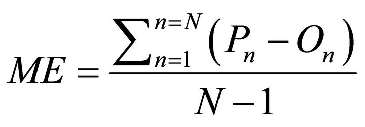
The ME (1) is given by the mean difference between the forecast and the observed values, indicating the systematic error. Positive error values express overestimation of the observed precipitation and negative values underestimation. When the forecast is perfect, the ME is equal to zero. The ME formula is:
 (1)
(1)
where Pn is the forecast value, On the observed one, and N the number of observations. The ME result has the same unity as the studied variable, in this case, millimeters of precipitation.
The other statistical parameter addressed on this work, is the RMSE (2), that is a frequently used measure of the difference between values predicted by a model and the values actually observed from the environment that is being modeled. These individual differences are also called residuals, and the RMSE serves to aggregate them into a single measure of predictive power. Unlike ME, this parameter gives information regarding the total amplitude of the error, disregarding the signal of positive or negative. The formula that defines the RMSE is:
 (2)
(2)
3. Results and Discussion
The error analyses are displayed in this section, preceded by a discussion about the main meteorological systems responsible for the spatial and temporal distribution of the accumulated precipitation in each month (Figure 1), where dark green color represents the largest amounts of precipitation. On the ME figures, positive values are represented by colors of red tones, and negative values by colors of blue tones. The dark red colors on the RMSE indicate larger errors.
During January 2012 it was observed the presence of three atmospheric mechanisms inductors of precipitation: the Intertropical Convergence Zone (ITCZ) [23-25] over the equatorial Atlantic; the South Atlantic Convergence Zone (SACZ) [26,27], extending from Southern Amazonia to Southeast Brazil, and Upper Tropospheric Cyclonic Vortices (UTCV) [28] over Northeast Brazil. These systems were responsible for a maximum of precipitation over Amapá and Pará (over 400 mm; Figure 1(a)), while the precipitation over Maranhão was reduced (less than 200 mm, except for the South of São Luís). Such pattern was due to the displacement of the UTCV to the Eastern Amazonia, which generates subsiding air and inhibition of precipitation over Maranhão.
The ME and RMSE of the models produced distinct results (Figure 2). The GFS scored the smallest relative values of ME during the forecast horizons, tending more to an underestimation of the precipitation. However, the

Figure 1. Acumulated precipitation (mm) over Eastern Amazon for: (a) January; (b) February; (c) March; (d) April, of 2012.
magnitude of the RMSE was larger, mostly over Pará. The BRAMS and ETA models, which overestimated the precipitation, show similar results regarding the RMSE, with higher values located on the border between Pará and Maranhão. Comparing these models, BRAMS and ETA scored the smallest RMSE. As for the forecast horizons, one can notice that the errors are systematic, so the same pattern seen for 24 h can be observed for 48 h.
During February 2012, the UTCV stopped influencing the weather and Frontal Systems (FS) advances to Southern Amazon was reduced. The ITCZ was therefore the main atmospheric system acting on the region, especially over northeastern Pará and Amapá. The highest precipitations were restricted to Marajó Island and northeastern Pará, where more than 400mm was recorded (Figure 1(b)). The development of Squall Lines (SL) along the Maranhão shore also contributed to the highest accumulated precipitation.
The spatial pattern of ME (Figure 3) shows that the GFS underestimates the precipitation over the north of Pará and Amapá, where the largest amounts of rain were recorded. On the other regions, the model shows ME near zero, which represents an accurate forecast.
In general, BRAMS and ETA presented more areas with under and overestimation errors. At Maranhão, where the total of accumulated precipitation ranged spatially between 150 mm and 350 mm, the RMSE was smaller than the other regions with high precipitation. The error magnitude was higher over Pará, for both forecasts horizons.
March is characterized by the peak of the rainy season (Figure 1(c)), so that many counties experiences extreme events. In addition, Northeastern Pará, Marajó Island and part of the Lower Amazon River received precipitation above the climatology, e.g. the total of precipitation at Belém was above 700 mm, in March 2012. The elevated sea surface temperature of the Atlantic contributed to sustain an intense ITCZ and FS started to impact Southern Amazonia.
With the rising of precipitation, RMSE and ME also increased (Figure 4). GFS continued to display underestimated values over Pará. Still, ETA and BRAMS displayed overestimation for the 24 h forecast, but it reduced for the 48 h horizon, mostly at Pará, Amapá and Northern Tocantins.
The RMSE analysis ratifies that GFS was the one with the largest errors on almost all region during March.

Figure 2. ME and RMSE of GFS (left column), BRAMS (middle column) and ETA (right cloumn) for the forecast of 24 h and 48 h. Mean of January of 2012.
BRAMS and ETA had a better performance; only Northern Pará and Maranhão shore displayed high values (above 20 mm). On the other regions, the less amount of precipitation was determinant for the small value of RMSE, mainly for the 24 h forecast.
It is noteworthy that March was a particularly rainy month, and GFS performance may have suffered from this anomaly. In addition, BRAMS and ETA predicted even higher values for areas with extreme events.
During April 2012 (Figure 1(d)), the ITCZ was virtually the only large-scale atmospheric system influencing Amazonia. Therefore, the most affected areas were in Northern Pará and Amapá, with accumulated values above 400 mm. With these systems displaced further North, other regions, such as the center of Maranhão, received small amounts of precipitation, with values below 150 mm.
The spatial distribution of ME continues the trend of

Figure 3. ME and RMSE of GFS (left column), BRAMS (middle column) and ETA (right column) for the forecast of 24 h and 48 h. Mean of February of 2012.
the other months of the rainy season (Figure 5). The GFS continues to underestimate the precipitation for the 24 h and 48 h forecasts, indicating that the model follows a climatological pattern. The worst performance of BRAMS occurred in April, when it overestimated precipitation in all Eastern Amazonia. One possible answer to BRAMS errors may be the fact that its output represents the mean value of the grid cell, while precipitation shows a high spatial variability [29]. ETA is also shown overestimation, especially in Maranhão, where the model overestimated the observed precipitation for both 24 h and 48 h forecasts.
The RMSE analysis shows that GFS scored the smallest values, mainly over Southeastern Pará, centersouth Maranhão and Northern Tocantins (Figure 5). Similar behavior could be noticed for BRAMS and ETA, where the highest values were in Pará and Amapá. The smallest values of error over Maranhão indicates that GFS repre-

Figure 4. ME and RMSE of GFS (left column), BRAMS (middle column) and ETA (right cloumn) for the forecast of 24 h and 48 h. Mean of March of 2012.
sented well the precipitation at this state, as well as in Northern Tocantins.
4. Conclusions
The ME and RMSE analyses, showed that none of the models could perfectly forecast precipitation in Eastern Amazonia. The BRAMS and ETA models displayed a tendency of overestimation of the observed precipitation, while GFS tended to underestimate it, mostly when the total amount of rain was above the climatology.
The regions with the highest errors for both forecast horizons were Lower Amazonas River, Marajó Island and Northeast Pará. Such results may be associated with the high precipitation during these four months; also in adtition, the density of rain gauges is low, making the interpolation of observed data more uncertain.
In general, the GFS showed good forecasts for Maranhão, Northern Tocantins and Southeast Pará. BRAMS and ETA also had good performances for the same regions, in spite of the tendency for overestimation.

Figure 5. ME and RMSE of GFS (left column), BRAMS (middle column) and ETA (right cloumn) for the forecast of 24 h and 48 h. Mean of April of 2012.
5. Acknowledgements
The authors would like to thank NOAA and CPTEC for the data, Vale Institute of Technology for the grants, equipment and physical structure for the development of this work, which was implemented under the “Integrated monitoring and forecasting of meteorological and hydrological events for Vale, in the Eastern Amazonia” Project.
NOTES