The Effect of Relaxation Time on the Heat Transfer and Temperature Distribution in Tissues ()
1. Introduction
Heat transfer in biological systems is relevant in many diagnostic and therapeutic applications that involve changes in temperature. For example, in hyperthermia the tissue temperature is elevated to 42˚C - 43˚C using ultrasound [1]. There has also been long standing interest in thermal properties of skin [2] in order to understand conditions leading to thermal damage (burns) to skin, usually involving contact of skin to hot objects [3], in which local thermal conduction and heat capacity are dominant. Spatially distributed heating of skin and deeper tissue by electromagnetic fields and ultrasound is also of established interest [4]. Many of the bioheat transfer problems have been modeled using the Penne’s equation, which accounts for the ability of tissue to remove heat by both passive conduction (diffusion) and perfusion of tissue by blood.
Prediction of heat transport has long been carried out by both analytical and numerical methods [5,6]. The temperature rise for constant (temperature independent) perfusion has been predicted by traditional analytical methods based on bioheat transfer equation, which can be solved analytically for simple geometries [7] or by finite element models for more realistic, complicated tissue geometry [8,9]. Models which include temperature-dependent increases in perfusion are more difficult to solve, but the case of linear temperature dependence have been described using analytical expressions [10] and numerical simulations [9]. The bioheat transfer equation has been used in a wide range of applications to describe heat transport in blood perfused tissues, [11] and solved by a variety of methods. An adaptive finite element method was used to optimize the nonlinear bio-heat equation for optimizing regional hyper-thermia [12]. Twodimensional bio-thermal models of ultrasound applicators based on the bio-heat equation were solved by finite difference equation [13]. The boundary element and finite difference methods have also been used to solve the bio-heat equation [14-18].
The normal mode method analysis gives exact solutions without any assumed restrictions on temperature distributions. It is applied to wide range of problems in different branches (Othman [19-21], Sharma et al. [22], Othman and Kumar [23], Othman and Singh [24] and Othman et al. [25]). It can be applied to boundary-layer problems, which are described by the linearized Navierstokes equations in electro-hydrodynamic (Othman [26]).
In this paper, the normal mode analysis can be employed to solve the bio-heat transfer equation analytically. The soft tissue is considered as a viscoelastic medium and the relaxation time has been used in the bio-heat transfer equation. It has enabled us to study the effects of relaxation time on heat transport in blood per θ (0, y, t), at x = 0 fused tissues.
2. Bio-Heat Transfer Equation
The temperature evaluation in biological tissues can be modeled with Penne’s bioheat equation, which is
 (1)
(1)
where, T is the temperature,  is the density of tissue, CT is the heat capacity of tissue, k is the diffusion due to blood flow,
  is the heat capacity of blood,
  is the perfusion due to blood flow,
  is the density of blood,
  is the arterial blood temperature, Q is the absorbed power density and
  is the relaxation time The following dimensionless parameters were defined as
 (2)
(2)
where, L is the tissue length.
Equation (1) can be rewritten in the following dimensional form
 (3)
(3)
3. The Normal Mode Analysis
The solution of Equation (1) can be decomposed in terms of normal mode as the following form
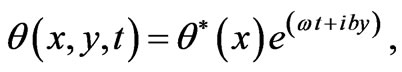 (4)
(4)
 (5)
(5)
where, b is the wave number in the y-direction,  is a complex time constant,
  and
and  are the amplitude of the functions
  and G respectively.
Substituting from Equations (4) and (5) into Equation (3) we obtain
 (6)
(6)
where

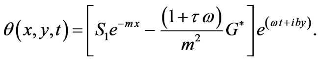
The solution of Equation (6) has the form
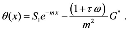 (7)
(7)
Then
 (8)
(8)
4. Boundary Conditions
 (9)
(9)
Substituting from Equations (4) and (8) into Equation (9) we obtain
 (10)
(10)
5. Computational Results
In the following calculations, the typical tissue and blood properties are applied as follow: ρ = 1000 Kg/m3, Cb = 4200 J/kg∙˚C, Tb = 0.01, k = 0.5W/m∙˚C, ωb = 0.5Kg/m3∙s.
Also, the values adopted to each dimensionless parameters employed in this work are given by G = 1.0, Tb = 0.01, and these values correspond to a tissue with characteristic dimension of 3 cm. Figure 1 shows the temperature distribution at different times as function of distance. It is clear from this figure that the tissue temperature at the early stage of heating decreases with increaseing the tissue depth. In this paper, the soft tissue can be treated as a viscous liquid for propagation of ultrasound. The amount of heat generated in tissue is most dependent on the absorption coefficient of the tissue. Acoustic absorption due to shear relaxation invariably can not be accounted for by single relaxation times instead a continuous distribution of relaxation times must be used. This is because the relaxation process arises from the finite time taken for molecules to diffuse between adja-

Figure 1. Temperature distribution as function of distance for different times (k = 0.5 W/m∙˚C, ωb = 0.5 Kg/m3∙s).

Figure 2. Temperature distribution as function of distance for different values of relaxation time (k = 0.5 W/m∙˚C, ωb = 0.5 Kg/m3∙s).
cent shearing layers in the medium [27]. The time taken for a particular molecule to diffuse depends upon its local environment which because of the random nature of medium is different for each molecule. Figure 2 shows the temperature distribution at different non-dimensional relaxation time as function of propagation distance. From this figure it can seen that the tissue temperature increases with the increase of the relaxation time.
Every person has a varied blood perfusion at various health statuses. Figure 3 depicts the tissue temperature responses corresponding to three different blood perfusion levels. For the case of , the tissue temperature appears much smaller than that of using
  at the same position. It can be seen that large blood perfusion tends to prevent the biological body from burn injury. Figure 4 shows the influence of the thermal conductivity on the tissue temperature response. The tissue temperature increases with the increase of the thermal conductivity of tissue. The temperature of the surface tissue will be closer to the body core temperature when the thermal conductivity becomes high enough. In fact, the thermal conductivity of the tissue depends on its components. The water in the tissue may affect the thermal conductivity of the respiratory tract. Usually, the thermal conductivity of tissue will decrease with the loss of water. This may imply that the thermal injury will be more serious if taking into concern the decrease of the thermal conductivity due to water loss. Figure 5 gives the temperature distribution in tissue, and depicted the surface tissue temperature increases immediately after the exposure, while in the deeper tissues, the temperature decreases slightly until after propagation in the x-y plane. The numerical results using normal mode analysis are in a good agreement with previously published data.

Figure 3. Effect of blood perfusion levels on temperature response as function of distance (k = 0.5 W/m∙˚C, t = 0.8).

Figure 4. Effect of thermal conductivity of tissues on temperature response as function of distance (ωb = 0.5 Kg/m3∙s, t = 0.8).

Figure 5. Temperature distribution in 3-D (k = 0.5 W/m∙˚C, ωb = 0.5 Kg/m3∙s, t = 0.8).
6. Conclusions
Closed form analytical solutions to the bioheat transfer problems with generalized spatial heating inside the biological bodies are investigated. Effects of the individual’s physiological variables (such as blood perfusion, thermal conductivity and relaxation time) were investigated in detail. The analytical solutions presented in this paper can be used to predicate the evolution of the detailed temperature within the tissues during thermal therapy. The present solution in this paper is very useful for a variety of bio-thermal studies.