Spatial Segregation Limit of a Quasilinear Competition-Diffusion System

Qunying Zhang^1*, Shan Zhang², Zhigui Lin¹

¹School of Mathematical Science, Yangzhou University, Yangzhou, China.
²School of Applied Mathematics, Nanjing University of Finance Economics, Nanjing, China.

DOI: 10.4236/am.2015.612175                

Abstract

The aim of this paper is to investigate a Volterra-Lotka competition model of quasilinear parabolic equations with large interaction. Some existence, uniqueness and convergence results for the system are given. Also investigated is its spatial segregation limit when the interspecific competition rates become large. We show that the limit problem is similar to a free boundary problem.

Keywords

Competition-Diffusion System, Quasilinear, Spatial Segregation, Free Boundary Problem

1. Introduction

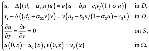
In this paper, we study the spatial and temporal behavior of interacting biological species. Assuming the reaction rates of competition follow the Holling-Tanner interaction mechanism, the quasilinear reaction-diffusion model under consideration can be given by

(1)

here, , , where is a bounded domain in. are all positive constants. and stand for their population densities of the competing species at the time t and at the habitat. is the respective intrinsic growth rates, and represent the intra-specific competition rates, whereas and represent the inter-spe- cific competition rates. The boundary condition models the fact that species have no-flux near the boundary, where is the outward normal unit vector to. may not be equal to from an ecological point of view, but for the convenience of presentation, we may assume here.

Quasilinear parabolic equations have received a great attention in recent years. We can refer to [1] -[6] and the references therein for more details. However, the main concerns in above works are for the existence of a global solution, a weak solution, periodic solutions, the existence-uniqueness of positive solutions, blow-up property of the solution, and the qualitative property of the solution including finite time extinction and large time behavior of the solution.

Our main interest is different from those of the above works, we mainly consider the spatial segregation limit of (1) when only the interspecific competition rates and are very large. To study this case, it is convenient to rewrite (1) as the following equivalent form:

(2)

where and k are positive constants derived from, and k is the only parameter which is large. For similar studies, here we refer [7] -[15] to the interested readers for more information. A striking difference between (2) and above relevant works is that the diffusion term in (2) is quasilinear. When and, the system (2) is reduced to the classical Volterra-Lotka competition model, which has been studied in [9] , where Dancer et al. showed that the two competition species spatially segregate as k tends to infinity. Moreover, they proved that, for any, there exist subsequences and of the k-dependent non- negative solutions converging weakly in to the positive and negative parts respectively of a limit function w satisfying a scalar equation of the form

(P)

where, , and they also showed that the limit problem (P) turns out to be an explicit Stefan-like type free boundary problem.

Motivated by [9] , our main purpose of this paper is to extend most of results of [9] to systems (2) with quasilinear diffusion terms. In addition, we will get the convergence results for the further improvement. Specifically, we have strong convergence in.

Note that the study of strong-competition limits in corresponding elliptic of parabolic systems is of interest not only for questions of spatial segregation and coexistence in population dynamics, as here and in [7] [9] [13] [16] -[19] but also is key to the understanding of phase separation in Hartree-Fock type approximations of systems of modelling Bose-Einstein condensates, see [10] [20] [21] [23] , and reference therein.

To conclude, we observe that a couple of problems addressed and solved for family of solutions to (2) remains for further study in our general context: firstly, to develop a common regularity theory for the solutions of the system, which is independent of the competition rate, as in [16] -[18] [21] [22] ; secondly, to study the regularity of the class of limiting profiles, both in terms of the densities and in terms of the emerging free boundary problem, as in [10] [16] [23] [24] ; thirdly, the precise description of the singular set in the emerging free boundary problem, as in [25] [26] . These will be object of future investigation.

The outline of this paper is arranged as follows. In Section 2, we give some a prior estimates and some convergence results for solutions of problem (2). Section 3 is focused on the limit problem as. In Section 4, we get the further convergence results in the special case of. Concluding remarks are given in the last section.

2. Preliminaries

In order to study the limit case as, we rewrite problem (2) as

(3)

Throughout this paper, we let and suppose the initial functions and satisfy

(4)

We say a pair is a solution of (3) in the sense that and satisfy (3). We now prove some basic facts of solutions for problem (3), which will be used later.

Lemma 1. The solution of problem (3) exists and is unique. Moreover, there exist constants and such that

Proof. The existence and uniqueness of solutions of (3) are followed from the standard parabolic equations theory [4] .

By using the maximum principle, the solution is positive for and. For the upper bound, it follows from the comparison principle that for, where

which is the solution of the problem

(5)

Thus we have

Similarly, there exists a constant such that

Lemma 2. Let be the solution of problem (3), then

(6)

where is a constant which is independent of k.

Proof. Integrating the equation for in (3) over and using Green’s formula yield

(7)

By Lemma 1 and noting that the right side of (7) is independent of k, we get (6).

Lemma 3. Let be the solution of problem (3), then

(8)

where is a constant which is independent of k.

Proof. Multiplying the equation for in (3) by, integrating over and applying Green’s formula, we yield

which leads to

where we have used Lemma 1. To get the first estimate of (8), we simply integrate the above inequality from 0 to T. The second inequality of (8) can be derived similarly.

In order to derive a free boundary problem, we also need to introduce a new function

which is related with. Then satisfies the scalar problem

(9)

(10)

(11)

The following result yields uniform boundedness of.

Lemma 4. The sequence is bounded in uniformly with respect to k.

Proof. Multiplying the Equation (9) with, and integrating over using integration by parts, we get

where is the duality product between the space and. By Lemmas 1 and 3, we then have

where M is a positive constant which is independent of k or. This implies

With the above discussion, below we study some convergence properties. It follows from Lemmas 1 and 3 that and are uniformly bounded in. Hence, there exist subsequences of and (still denoted by and), and two functions such that

(12)

and

(13)

as. Furthermore, by Lemma 2, we have

Lemma 5. a.e. in.

Below we manage to build the relations between u, v and w.

Lemma 6. The subsequences and are such that

(14)

as, where and. Moreover,

(15)

Proof. Let be such that

In order to prove the theorem, we need to divide our proof into three cases:

In case, according to the definition of limit, there exists a positive constant such that

then we have

Due to Lemma 2, above inequality implies that

Next we consider case. We proceed as in the proof of case (a), then there exists a positive constant such that

Recalling Lemma 2, we claim that

For the last case. We claim that

Otherwise, if there is a subsequence of, which we still denote by, such that, it follows that, consequently, which contradicts the fact. Similarly, it is impossible to have that.

From the boundedness of and, it is easy to achieve convergence in. To the end, we get (15) from (14).

3. The Limit Problem as

Lemma 6 illustrates that and weakly in as. We set

(16)

and

(17)

In this section, we mainly consider the scalar equation

(18)

First, we show that problem (18) has a weak solution, which are defined as follows:

Definition 3.1 We say that a function is a weak solution of (16) if it satisfies

(19)

for all and any test function with.

Theorem 1. The function defined by (15) is the unique weak solution of problem (18). Moreover, for some.

Proof. From Lemmas 1 and 3, we easily have, and Lemma 4 yields. is derived from by a standard regularity result (see for example [27] , Theorem 3, p.287).

Multiplying (9) by a test function with, and using integration by parts, we deduce

Let along the sequence for which (12) holds. By the dominated convergence theorem and Lemma 1, we have

(20)

Note that (16) and (17) yield

and

With (20), we then have that z satisfies

for all and any test function with. Namely, z satisfies the differential equation in (18) as well as the homogeneous Neumann boundary condition in the sense of distributions, and the initial condition

This follows easily that z is the weak solution of problem (18).

It is clear from [2] that the weak solution of problem (18) is unique. Last, for the regularity of z, we refer to Theorems 1.1 and 1.3 in [28] .

According to the above discussion, there exists a family of closed hypersurfaces , which separates the two strongly competing species. That is

and

We denote

Finally, as in [9] , we rewrite a strong form of the limit problem (18), where the equations can be described a classical two-phase Stefan-like free boundary problem.

Theorem 2. Let z be a weak solution of limit problem (18), if is smooth enough, and if the functions

are smooth up to, then u and v satisfy

(21)

where we suppose that.

4. Further Convergence Results

In this section, we prove that the subsequences and of k-dependent non-negative solutions to (3) converge strongly in. For the convenience of presentation, we consider the special case of.

Theorem 3. If and a.e. in, then up to a subsequence,

(22)

and hence in, in, in.

Proof. By arguments as in the proof of Theorem 1, we first obtain

Thus

This implies

by Lemma 7.6 in [29] . Hence Also by Lemma 7.7 in [29] and Lemma 5, we get

(23)

Now, multiplying the second equation in (3) by the limit u and integrating it over, , we

have

Integrating by parts gives

(24)

Integrating (24) with respect to over gives

With (4), (12) and Lemma 5, as, we obtain

and

Since is bounded in and a.e. in, we may apply Fubini theorem to obtain

(25)

as. Similarly, by (12), (23) and Lemma 5, we have

Therefore, (24) yields

This implies that

(26)

Next, multiplying the first equation in (3) by the limit u and integration it over, we have

(27)

Integrating above equation in and passing to the limit as yield

(28)

by using (4), (12) and (26).

Finally, multiplying the first equation in (1) again by and integrating it over, we deduce

This concludes that

(29)

by (28). It follows from (12) and weak lower semi-continuity that

By Fatou’s lemma, we have

which together with (29) implies that there exists a subsequence, which we denote again by such that for a.e.

In other words,

Hence in. Similarly, we claim that in. The rest of the conclusions in this theorem follow consequently.

5. Concluding Remarks

The study of spatial behavior of the interacting species has been attracting much attention in population ecology, in particular, in the case when the interactions are large and of competitive type. Many different models based on partial differential equations can be successfully employed to investigate the phenomenon of coexistence and exclusions of competing species. In this paper, we have attempted to study a class of quasilinear parabolic system (3) describing a Holling-Tanner’s competitive interaction of two species. We prove that if inter-specific competition rates tend to infinity, then spatial segregation of the densities and a scalar limit problem (21) are given. In particular, we have obtained the strong convergence results in in the special case of. Ecologically, our results show that competition leads to segregation.

Finally, we want to mention that there are still many interesting questions to do for this kind of problem. First of all, noting that the diffusion term of the first equation in (2) can be written as, the term describes the “self-diffusion”. Naturally to ask whether our results can be extended to parabolic systems with “cross-diffusion”? Moreover, as mentioned in the introduction, we have seen that limit profiles of solutions to (2) are segregated configurations, it is then natural to define the free boundary as the nodal set. The regularity of the nodal set remains a challenge, and it will be the object of a forthcoming paper.

Acknowledgements

We thank the Editor and the referee for their comments. This work is partially supported by PRC grant NSFC 11501494 and NSF of the Higher Education Institutions of Jiangsu Province (12KJD110008). This support is greatly appreciated.

NOTES

^*Corresponding author.

Conflicts of Interest

The authors declare no conflicts of interest.

References

[1]	Amann, H. (1990) Dynamic Theory of Quasilinear Parabolic Systems II. Reaction-Diffusion Systems, Differential Integral Equations, 3, 13-75.
[2]	Aronson, D.G., Crandall, M.G. and Peletier, L.A. (1982) Stabilization of Solutions oa a Degenerate Nonlinear Diffusion Problem. Nonlinear Analysis, 6, 1001-1022. http://dx.doi.org/10.1016/0362-546X(82)90072-4
[3]	Constantin, A., Escher, J. and Yin, Z. (2004) Global Solutions for Quasilinear Parabolic Systems. Journal of Differential Equations, 197, 73-84. http://dx.doi.org/10.1016/S0022-0396(03)00165-7
[4]	Ladyzenskaja, O.A., Solonnikov, V.A. and Ural’ceva, N.N. (1968) Linear and Quasi-Linear Equations of Parabolic Type. Transactions of the American Mathematical Society, Monographs 23, Providence.
[5]	Pao, C.V. (2007) Quasilinear Parabolic and Elliptic Equations with Nonlinear Boundary Conditions. Nonlinear Analysis, 66, 639-662. http://dx.doi.org/10.1016/j.na.2005.12.007
[6]	Zhang, Q.Y. and Lin, Z.G. (2010) Periodic Solutions of Quasilinear Parabolic Systems with Nonlinear Boundary Conditions. Nonlinear Analysis, 72, 3429-3435. http://dx.doi.org/10.1016/j.na.2009.12.026
[7]	Crooks, E.C.M., Dancer, E.N., Hilhorst, D., Mimura, M. and Ninomiya, H. (2004) Spatial Segregation Limit of a Competition Diffusion System with Dirichlet Boundary Conditions. Nonlinear Analysis: Real World Applications, 5, 645-665. http://dx.doi.org/10.1016/j.nonrwa.2004.01.004
[8]	Dancer, E.N. and Du, Y.H. (1994) Competing Species Equations with Diffusion, Large Interactions, and Jumping Nonlinearities. Journal of Differential Equations, 114, 434-475. http://dx.doi.org/10.1006/jdeq.1994.1156
[9]	Dancer, E.N., Hilhorst, D., Mimura, M. and Peletier, L.A. (1999) Spatial Segregation Limit of a Competition-Diffusion System. European Journal of Applied Mathematics, 10, 97-115.
[10]	Dancer, E.N., Wang, K. and Zhang, Z. (2012) The Limit Equation for the Gross-Pitaevskii Equations and S. Terracini’s Conjecture. Journal of Functional Analysis, 262, 1087-1131. http://dx.doi.org/10.1016/j.jfa.2011.10.013
[11]	Namba, T. and Mimura, M. (1980) Spatial Distribution for Competing Populations. Journal of Theoretical Biology, 87, 795-814. http://dx.doi.org/10.1016/0022-5193(80)90118-6
[12]	Shigesada, N., Kawasaki, K. and Teramoto, E. (1979) Spatial Segregation of Interacting Species. Journal of Theoretical Biology, 79, 83-99. http://dx.doi.org/10.1016/0022-5193(79)90258-3
[13]	Wang, K.L. and Zhang, Z.T. (2010) Some New Results in Competing Systems with Many Species. Annales de l’Institut Henri Poincare (C) Non Linear Analysis, 27, 739-761. http://dx.doi.org/10.1016/j.anihpc.2009.11.004
[14]	Wei, J.C. and Weth, T. (2008) Asymptotic Behaviour of Solutions of Planar Elliptic Systems with Strong Competition. Nonlinearity, 21, 305-317. http://dx.doi.org/10.1088/0951-7715/21/2/006
[15]	Zhang, S., Zhou, L., Liu, Z.H. and Lin, Z.G. (2012) Spatial Segregation Limit of a Non-Autonomous Competition-Diffusion System. Journal of Mathematical Analysis and Applications, 389, 119-129. http://dx.doi.org/10.1016/j.jmaa.2011.11.054
[16]	Caffarelli, L.A., Karakhanyan, A.L. and Lin, F.H. (2009) The Geometry of Solutions to a Segregation Problem for Nondivergence Systems. Journal of Fixed Point Theory and Applications, 5, 319-351. http://dx.doi.org/10.1007/s11784-009-0110-0
[17]	Dancer, E.N., Wang, K.L. and Zhang, Z.T. (2011) Uniform Hölder Estimate for Singularly Perturbed Parabolic Systems of Bose-Einstein Condensates and Competing Species. Journal of Differential Equations, 251, 2737-2769. http://dx.doi.org/10.1016/j.jde.2011.06.015
[18]	Conti, M., Terracini, S. and Verzini, G. (2005) Asymptotic Estimates for the Spatial Segregation of Competitive Systems. Advances in Mathematics, 195, 524-560. http://dx.doi.org/10.1016/j.aim.2004.08.006
[19]	Zhang, S., Zhou, L. and Liu, Z.H. (2013) The Spatial Behavior of a Competition Diffusion Advection System with Strong Competition. Nonlinear Analysis: Real World Applications, 14, 976-989. http://dx.doi.org/10.1016/j.nonrwa.2012.08.011
[20]	Chang, S.M., Lin, C.S., Lin, T.C. and Lin, W.W. (2004) Segregated Nodal Domains of Two-Dimensional Multispecies Bose-Einstein Condensates. Physica D: Nonlinear Phenomena, 196, 341-361. http://dx.doi.org/10.1016/j.physd.2004.06.002
[21]	Noris, B., Tavares, H., Terracini, S. and Verzini, G. (2010) Uniform Hölder Bounds for Nonlinear Schrödinger Systems with Strong Competition. Communications on Pure and Applied Mathematics, 63, 267-302.
[22]	Soave, N. and Zilio, A. (2015) Uniform Bounds for Strongly Competing Systems: The Optimal Lipschitz Case. Archive for Rational Mechanics and Analysis, 218, 647-697. http://dx.doi.org/10.1007/s00205-015-0867-9
[23]	Caffarelli, L.A. and Lin, F.H. (2008) Singularly Perturbed Elliptic Systems and Multi-Valued Harmonic Functions with Free Boundaries. Journal of the American Mathematical Society, 21, 847-862. http://dx.doi.org/10.1090/S0894-0347-08-00593-6
[24]	Tavares, H. and Terracini, S. (2012) Regularity of the Nodal Set of Segregated Critical Configurations under a Weak Reflection Law. Calculus of Variations and Partial Differential Equations, 45, 273-317. http://dx.doi.org/10.1007/s00526-011-0458-z
[25]	Caffarelli, L.A. and Lin, F. (2010) Analysis on the Junctions of Domain Walls. Discrete and Continuous Dynamical Systems, 28, 915-929.
[26]	Zhang, S. and Liu, Z.H. (2015) Singularities of the Nodal Set of Segregated Configurations. Calculus of Variations and Partial Differential Equations, 54, 2017-2037. http://dx.doi.org/10.1007/s00526-015-0854-x
[27]	Evans, L.C. (1998) Partial Differential Equations. Graduate Studies in Mathematics, Vol. 19, American Mathematical Society, Providence.
[28]	Dibenedetto, E. (1993) Degenerate Parabolic Equations. Springer-Verlag, New York. http://dx.doi.org/10.1007/978-1-4612-0895-2
[29]	Gilbarg, D. and Trudinger, N.S. (2001) Elliptic Partial Differential Equations of Second Order. 2nd Edition, Springer, New York.