A Solution of Kepler’s Equation

John N. Tokis^*

Technological Educational Institute of Epirus, Ioannina, Greece.

DOI: 10.4236/ijaa.2014.44062                

Abstract

The present study deals with a traditional physical problem: the solution of the Kepler’s equation for all conics (ellipse, hyperbola or parabola). Solution of the universal Kepler’s equation in closed form is obtained with the help of the two-dimensional Laplace technique, expressing the universal functions as a function of the universal anomaly and the time. Combining these new expressions of the universal functions and their identities, we establish one biquadratic equation for universal anomaly (χ) for all conics; solving this new equation, we have a new exact solution of the present problem for the universal anomaly as a function of the time. The verifying of the universal Kepler’s equation and the traditional forms of Kepler’s equation from this new solution are discussed. The plots of the elliptic, hyperbolic or parabolic Keplerian orbits are also given, using this new solution.

Keywords

Keplerian Motion, Universal Kepler’s Equation, Universal Anomaly, Two-Dimensional Laplace Transforms

1. Introduction

In the Keplerian problem, a body of mass follows a conic orbit, for which the focus is identified to the center of attracting body (with mass). The Keplerian motion is described by the fundamental differential equation of the physical two-body problem:

(1)

where is the vector position of the moving body related to the attraction center and the gravitational parameter defined by 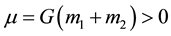(where the Newtonian gravitational constant) (see [1] , Equation (6.2.3)).

The traditional form of Kepler’s equation, which can be obtained directly from Equation (1) (see [1] , Section 6.3 and [2] ), is normally written as:

For elliptic orbits

(2a)

for hyperbolic orbits

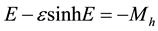(2b)

where is the eccentricity, the eccentric anomaly and the mean anomaly, which is defined as

(2c)

(2d)

(2e)

(see [2] , Equation (11) and [3] , Equations (4.35) and (4.51)). Remark that the time is measured from pericenter and is the semimajor axis, which is positive for ellipses, negative for hyperbolas, and infinite for parabolas; also, is the pericenter distance of the orbit. The case of leads to a circular orbit and the simple solution (cf., Equation (2a)), so that we will regard hereafter in the present work.

Johannes Kepler announced the relevant laws of above equation early in 1609 and 1619 [4] . He has used physics as a guide in this discovery [5] . For four centuries, the Kepler’s problem is to solve the nonlinear Kepler’s Equation (2) for the eccentric anomaly.

Early analytical solution of Kepler’s equation was considered in a comprehensive study of Tisserand [6] . Recently, analytical works of the solution and use of Kepler’s equation have been proposed by various authors (see, e.g., [7] - [12] ).

In virtually every decade from 1650 to the present, there have appeared papers devoted to the solution of this Kepler’s equation. Its exact analytical solution is unknown, and therefore, efficient procedures to solve it numerically have been well discussed in many standard text books of Celestial Mechanics and Astrodynamics as well as in a large number of papers. Colwell [13] contains extensive references to the Kepler problem in his book. During last two decades, studies were carried out by several investigators of the present problem [2] [14] -[18] . In these studies, they used numerical or approximations methods for solution of the Kepler’s equation. Hence, it appears that an analytical solution of the Kepler’s equation will be of great interest.

In the current study, an analytical investigation of the Kepler’s equation real roots in closed form is presented. In Section 2, we will establish the general form of Kepler’s equation and will clear up the useful identities of the universal functions. In Section 3, using the two-dimensional Laplace transform technique, we will present an analytical solution for the universal Kepler’s equation, obtaining the universal functions as function of the universal anomaly and the time. In Section 4, in the first step we will establish one new biquadratic equation for universal anomaly for all conics with the help of Newman’s equation (cf. Equation (23)) and some identities of the new expressions of universal functions. Then, the solution of the present problem has been obtained, solving this biquadratic equation for all conics.

Finally, discussion of the results, thus obtained, is presented in Section 5; the new solution of the problem will prove that verifies the traditional form of Kepler’s equations for elliptic, hyperbolic or parabolic orbits. The elliptic, hyperbolic or parabolic Keplerian motion is easily plotted, using this new solution.

2. General Form of Kepler’s Equation

In order to solve the Kepler’s Equation (2), we use here the generalized form of this equation with the universal functions and the universal anomaly instead of the eccentric anomaly (see [3] , Section 4.5).

Working for the Kepler’s Equation (2), we consider an object following a path of same eccentricity about the center of attracting body; the object is at time in (vector) position with (vector) velocity. The time t is measured from the pericenter passage; so, when this object was at position (with) of the pericenter with velocity (with) and eccentric anomaly. We emphasize that the vectors and originate at the center of attraction. Then, we introduce the universal anomaly, which is defined by Sundman transformation:

(3)

(see [3] , Equation (4.71)) and related to the classical eccentric anomaly by

(4a)

(4b)

(4c)

where E is the eccentric anomaly angle of elliptic or hyperbolic orbit and D the parabolic eccentric anomaly of parabolic orbit with dimension (see [9] , Equation (18)). The denotes the reciprocal of the semimajor axis, namely

(5a,b,c)

Depending on the sign of or the value of the eccentricity, the type of the orbit is determined such that: (or) for elliptic orbits; (or) for hyperbolic orbits and (or) for parabolic orbits. Note that the universal anomaly is a new independent variable with dimension (see [3] , Equation (4.70)).

From the initial condition and the known relations:, for elliptic orbits and, for hyperbolic orbits (see [3] , Sections 4.3 and 4.4), we have also for the present problem

(6a,b)

where stands for the pericenter distance of the orbit related to the parameter with the relation

(7)

Remark that the is a non-negative parameter and the pericenter distance may be positive or zero; both of them have dimensions of length (see [3] , Section 4.1).

Now, using the universal functions defined by

(8)

with their following useful properties:

(9a)

(9b)

(9c)

(9d)

(see [3] , Equation (9.73)), the two forms of Kepler’s Equation (2) are incorporated in one universal equation

(10)

which is a standard form of the traditional Kepler’s Equations (2) with the epoch at pericenter passage (see [9] , Equation (23) and [2] , Equation (29)). The general formula (10) is valid for all values of and; in particular, it is good for parabolic orbits where.

To find out the expression of many orbital quantities, e.g. the magnitude of the position vector, we must solve the standard universal form (10) of the Kepler’s equation for the universal anomaly as function of the time, namely.

3. Solution of the Universal Kepler’s Equation

In order to obtain the analytical solution of the present problem, we shall solve first the universal Kepler’s equation Equation (10), obtaining the universal functions, as a function of the universal anomaly and the time. For this purpose, we will use the double Laplace transformation technique, which was analytically studied by Aghili and Salkhordeh-Moghaddam [19] and by Valkó and Abate [20] .

The universal functions: For this case, we introduce a new variable so that

(11a)

(11b)

(11c)

(see Equations (9)) and the universal Kepler’s Equation (10) becomes

(12a)

From the initial condition or and Equation (9a), we have the corresponding initial conditions to the Equation (12a)

(12b)

The application of double Laplace transform (with respect to and) to the Equations (12) gives the solution in transform domain as

(13)

where and are the transform variables of and time, respectively. For the solution of partial differential Equation (12a), we use the Appendix.

Now, the universal function can be obtained by taking the inverse transform of Equation (13) (cf., Appendix). So, we get

(14)

where we have abbreviated

(15)

with dimensions:.

The universal functions: For this case, we will use a new variable so that

(16a)

(16b)

(16c)

(see Equations (9c)) and the universal Kepler’s Equation (10) becomes

(17a)

For or and Equation (9a), we have the initial conditions to the Equation (17a)

(17b)

Similarly as in the case of, using the double Laplace transform (with respect to and) for the Equations (17), we obtained the solution in transform domain as

(18)

(cf., Appendix). Inverting we have the universal function

(19)

where we have defined the non-dimensional function

(20)

Then, substituting the results of Equation (14) and (19) into the relations and (cf., Equation (9b)), respectively, we can easily obtain the new universal functions and as

(21)

(22)

where and are given from Equations (15) and (20), respectively.

4. Analytical Solution of the Problem

In order to obtain a solution for the universal anomaly, we use the explicit expression for:

(23)

where. This relation was discovered by C. M. Newman and its does not involve any of the universal functions (see [3] , Equation (4.86)). The can be also given by the known equation (see [3] , Equation (4.83))

(24)

Substituting Equation (24) (with given by (21)) into Equation (23), the following relation is obtained

(25)

To find out two more relations between, and, similar to Equation (25), we will use the basic relation and the definitions of and Equations (15) and (20), respectively. Thus, we can easily obtain the relation

(26)

Further, we can find one more relation using the basic identity (see [3] , Equation (4.93)); indeed, with the help of Equations (14), (21) and (22), we obtain the relation

(27)

The three Equations (25), (26) and (27) are a system of the three unknowns:, and. Solving this system, we get from two Equations (25) and (26) the following relations

(28a)

(28b)

Finally, substituting Equations (28) into Equation (27), we obtain the following biquadratic equation for universal anomaly

(29)

where we have abbreviated

(30a)

(30b)

(30c)

with dimensions:, and.

The solution of the biquadratic Equation (29) gives the relation between the universal anomaly and the time for all conics: ellipse, hyperbola or parabola. The solution of this equation can be obtained using the standard formula of the solution for biquadratic equation.

Solving the new biquadratic Equation (29), we get the solution of the present problem for the universal anomaly at time as shown below

(31)

where we have abbreviated

(32a)

particularly, for elliptic orbits we have

(32b)

for hyperbolic orbits

(32c)

and for parabolic orbits

(32d)

Remark that the discriminant of the biquadratic Equation (29) is, for. Consequently, the solution (31) is real in the cases of hyperbolic and parabolic cases since the corresponding, given from Equations (32c,d), are always real-valued. In the case of the elliptic Keplerian orbits, the Equation (31) is real only in the special case for which, given from Equation (32b), becomes real, namely for the case

(32e,f)

where is the mean anomaly defined by Equation (2c). The upper limit of this mean anomaly is defined from the relation (32f) for every completed trip of the orbiting body in its elliptic orbit about the center of the attracting body; this limit is useful for determination of each Keplerian ellipse (cf., the applications in the next section).

In the case of parabolic orbits where the limiting case (or) and corresponds to and, the equation (29) and its solution (31) are reduced to

(33a)

(33b)

The Equation (31) is the solution of the present problem for all conics (ellipse, hyperbola or parabola) and expresses the relation between the universal anomaly and the time t.

Knowing the solution of the universal anomaly, we establish the exact expressions of the universal functions, n = 0, 1, 2, 3 as functions of the time. Indeed, using Equation (31), the Equation (28) are obtained as functions of the time:

(34a)

(34b)

Then, the universal functions (19), (14), (21) and (22) are expressed as functions of the time t as show below

(35a)

(35b)

(35c)

(35d)

The magnitude of the position vector of the orbiting body is

(36a,b)

(see [3] , Equation (4.82) and [14] , Equation (8)). Substituting into Equation (36b) the new expressions of, given by Equation (35b), we obtain the time-dependent distance of the orbiting body from the center of attraction as

(37)

Furthermore, if we work in the orbital reference system with the origin at the attracting center (or focus), we chose the plane to be the plane of motion with -axis pointing toward pericenter and -axis in the direction for which the true anomaly is 90˚; in this way the -axis is parallel to the angular momentum. Then, if and are the coordinates of a point on the conic orbit, we have and

(38)

where is the non-negative quantity given by Equation (7) (see [3] , Equation (4.3)). Thus, the and coordinates can be expressed as function of the time, using Equations (38) and the identities:,; namely, we get

(39a)

(39b)

where and are given from Equations (35) (see [14] , Equations (6)-(7)).

5. Discussion

Using the standard form of the universal Kepler’s equation (10) with the epoch at pericenter passage, we have derived a new biquadratic equation (29) for universal anomaly as a function of the time. This equation governs the motion of an orbiting body following a path with position vector from the center of attracting body and with velocity vector.

The new solution (31) of the present problem was obtained solving Equation (29) with initial-value conditions for the orbiting body at time passages from the pericenter, with minimum position vector, velocity vector and eccentric anomaly.

The solution (31) is a solution of the present problem. Indeed, the new expressions of the universal functions, and given by (35a,c) verify universal Kepler’s Equation (10). Moreover, the solution (31) is a solution of the Equation (29), since it can be easily verified by substitution of (31) into (29).

The solution (31) verifies also the traditional forms of Kepler’s Equation (2). Particularly, in the case of elliptic orbits the solution (31) of the problem is reduced for the eccentric anomaly (cf. Equation (4a)) to the form

(40)

where is the mean anomaly given by Equation (2c) and

(41)

Note that and (cf. Equation (32f)) for.

Similarly, in the case of hyperbolic orbits the solution (31) of the problem is reduced, for the eccentric anomaly (cf. Equation (4b)), to

(42)

where is the mean anomaly given by Equation (2d) and

(43)

Finally, in the case of parabolic orbits the solution (33b) gives for the parabolic eccentric anomaly (cf. Equations (4c) and (2e)):

(44)

From the other hand, the standard and hyperbolic trigonometric functions of Equations (2) are expressed as

(45a)

(45b)

where we have use Equation (35) and the relationship between the function U₁ and the standard and hyperbolic

trigonometric functions of Equations (2): and for ellipse

and hyperbola, respectively (see [3] , Problem 4 - 21 and [9] , Equation (24)).

Now, we will prove that the Equations (40) and (42) represent the solutions of the traditional forms of Kepler’s Equations (2). Indeed, it can be shown that the left-hand sides of Equations (2) are reduced to the right- hand sides, namely

(46a)

(46b)

in accordance with the Equations (40), (42) and (45).

It should be pointed out that our solutions for eccentric anomaly (cf., Equations (40) and (42)) are ready for physical applications in the corresponding Keplerian orbits.

In addition to above Keplerian orbits, the new solution (33b) of the present problem for the case of parabola (and) verifies the traditional Barker’s equation for parabolic orbits

(47)

Remark that the parabolic Keplerian equation is called Barker’s equation (see [3] , Equation (4.24)). Indeed, from the definition (8) for the universal functions we have and. Using the solution (33b), these universal functions are expressed from Equations (35a,c), so that

(48a,b)

where is given from Equation (32d). Then, the left-hand side of Equations (47) is reduced to the right- hand side, namely

(49)

In order to study the Keplerian orbits with the help of the new solutions, we use also the cartesian coordinates and with the origin at the center of the ellipse or hyperbola. In this case the and coordinates of the orbital plane system given by Equations (39) are related to the system with the relations and (see [3] , Equation (4.4)); so, for the case, these new coordinates can be obtained in the explicit forms

(50a)

(50b)

where we have defined the non-dimensional relation

(51)

in accordance to the Equations (39). Then, we introduce the non-dimensional coordinates

(52a)

(52b)

The new expressions (52) verify the following equations of ellipse and hyperbola, respectively:

(53a)

(53b)

where is defined by Equation (51). Remark that the equations (53) are the non-dimensional forms of the ellipse and hyperbola, respectively, in the cartesian system with the origin at the center of the ellipse or hyperbola (see [1] , Equations (A.2.1) and (A.4.2)).

In the other hand, for the case of parabola, the coordinates and can be also obtained, from Equations (39), as following

(54a)

(54b)

Then, we have, from Equations (54),

(55a,b)

The last Equation (55) is the equation of parabola, which passes through its pericenter with coordinates

(see [3] , Equation (3.22)). The non-dimensional form of Equation (55) is

(56)

with the non-dimensional coordinates

(57a,b)

In addition to above results for the non-dimensional coordinates we have (for physical application) the corresponding expressions:

For elliptic orbits the Equation (51) becomes

(58a)

for hyperbolic orbits the Equation (51) becomes

(58b)

for parabolic orbits the Equation (57a) yields

(58c)

where, and are the mean anomalies of ellipse, hyperbola and parabola, respectively (cf., Equations (2c,d,e)). These mean anomalies can be varied from 0 to, where is an integer. Note that the non- dimensional coordinates of attractive center (or focus) in the non-dimensional cartesian system is given by for all Keplerian orbits (ellipse, hyperbola or parabola).

In order to get a physical insight into the new solution of the Kepler’s problem, we apply the above results for the system Earth-Moon. For this system the eccentricity of the Moon is and the upper limit for the mean anomaly can be obtained from relation (32f) as. So, varying the mean anomaly (with) and using Equations (58a) and (52b), the elliptic Keplerian motion of the Moon about the Earth can be easily plotted in the non-dimensional cartesian system (Figure 1). Remark that the non-dimen- sional coordinates of the Earth are obtained as.

Note that the use of the upper limit of the mean anomaly, given from the relation (cf. relation (32f)), is import for the plotting of all elliptic Keplerian orbits. To confirm that we give two more examples: (a) We consider an object following an elliptic orbit with eccentricity about the center of attracting body; the upper limit of the mean anomaly, from relation (32f), is; then, varying the mean anomaly (with) and using Equations (58a) and (52b), we plot the elliptic Keplerian orbit in the non-dimensional cartesian system (Figure 2). (b) We consider another object in an elliptic orbit with

Figure 1. The elliptic orbit of the Moon about the Earth.

Figure 2. Two elliptic Keplerian orbits with eccentricities and.

eccentricity about the center of another attracting body; the upper limit of the new mean anomaly, from relation (32f), is; and, varying the mean anomaly (with), we plot the elliptic Keplerian orbit in the non-dimensional cartesian system (Figure 2).

Now, varying the mean anomaly (with for the present plot) and using equations (58b) and

(cf., Equation (52b), we plot of the hyperbolic Keplerian motion of an orbiting body

with the eccentricity about the attractive center (Figure 3).

Finally, varying the mean anomaly (with for the present plot) and using Equations (58c), and (56), we plot of the parabolic Keplerian motion of an orbiting body with the eccentricity about the attractive center (Figure 4).

6. Conclusions

This work presents a solution to the well known Keplerian two body physical problem. From the investigation

Figure 3. The hyperbola of an orbiting body (with) about the attractive centre.

Figure 4. The parabola of an orbiting body (with) about the attractive centre.

for this new solution, the main conclusions have been drawn as following:

1) An analytical solution for the universal Kepler’s equation has been determined, obtaining the universal functions, n = 0, 1, 2, 3 as function of the universal anomaly and the time with the help of the two-dimensional Laplace transform technique.

2) Using an explicit expression for the universal anomaly without any of the functions (cf., Equation (23)) and some identities of the new obtained universal functions, we developed a biquadratic equation for universal anomaly for all conics: ellipse, hyperbola or parabola.

3) The solution of the present problem has been obtained, solving this biquadratic equation for all conics.

4) This new analytical solution for the universal anomaly has been discussed and proved that verifies the universal Kepler’s equation (cf., Equation (10)), since the time depended universal functions U₃ and U₁ verify this equation. Then, the solutions for the eccentric anomaly (cf., Equations (40) and (42)) were also proved that verify the traditional form of Kepler’s equations for elliptic or hyperbolic orbits. This new solution for the universal anomaly has also proved that verifies the traditional Barker’s equation for parabolic orbits [11] . The elliptic, hyperbolic or parabolic Keplerian motion is plotted, using this analytical solution.

5) To our knowledge, this work gives in closed form the actual analytical solution of the Kepler’s problem. The advantage of the new solution is simple and ready for physical applications in the elliptic, hyperbolic or parabolic Keplerian orbits.

Appendix

Solution of partial differential equations using two-dimensional Laplace transforms

The general form of second-order linear partial differential equation in two variables is given as following

(A1)

where are constants and is source function of and or constant. We use also the abbreviations for the initial conditions

(A2)

and their one-dimensional Laplace transformations, , and, where “” and “” the transform variables of and, respectively (see [19] and [21] for details). Then, we get the relations for two-dimensional Laplace transforms

(A3a)

(A3b)

(A3c)

(A3d)

(A3e)

(A3f)

(A3g)

(A3h)

(A3i)

in accordance with the two-dimensional analysis formula, which can be written as one-dimensional analysis in the direction followed by one-dimensional analysis in the direction:

(A4)

Now, applying double Laplace transformation to both sides of Equation (A1) and using Equations (A3), we obtain the solution of Equation (A1) in the transform domain as

(A5a)

with the abbreviation

(A5b)

In order to invert this two-dimensional Laplace transform, we follow the double inversion as a two- step process [20] . In the first step we invert, say, on the “” transform variable

(A6)

where we keep the second transform variable as a constant. In the second step we invert on the “” transform variable and obtain, finally,

(A7)

Conflicts of Interest

The authors declare no conflicts of interest.

References

[1]	Dandy, J.M.A. (2003) Fundamentals of Celestial Mechanics. 2nd Edition, Willmann-Bell, Virginia.
[2]	Fukushima, T. (1999) Fast Procedure Solving Universal Kepler’s Equation. Celestial Mechanics and Dynamical Astronomy, 75, 201-226. http://dx.doi.org/10.1023/A:1008368820433
[3]	Battin, R.H. (1999) An Introduction to the Mathematics and Methods Astrodynamics. Revised Edition, AIAA Education Series, New York. http://dx.doi.org/10.2514/4.861543
[4]	Voelkel, J.R. (2001) The Composition of Kepler’s Astronomia Nova. Princeton University Press, New York. http://press.princeton.edu/titles/7187.html
[5]	Bruce, S. (1987) Kepler’s Physical Astronomy. Springer-Verlag, New York.
[6]	Tisserand, F. (1894) Mecanique Celeste. Vol. 3. Gauthier-Villars, Paris.
[7]	Siewert, C.E. and Burniston, E.E. (1972) An Exact Analytical Solution of Kepler’s Equation. Celestial Mechanics, 6, 294-304. http://link.springer.com/article/10.1007/BF01231473#page-1
[8]	Tokis, J.N. (1973) Effects of Tidal Dissipative Processes on Stellar Rotation. PhD Thesis, Victoria University of Manchester, Manchester.
[9]	Fernandes, S.daS. (2003) Universal Closed-form of Lagrangian Multipliers for Coast-Arcs of Optimum Space Trajectories. Journal of the Brazilian Society of Mechanical Sciences and Engineering, 25, 1-9. http://dx.doi.org/10.1590/S1678-58782003000400004
[10]	Condurache, D. and Martinusi, V. (2006) Vectorial Regularization and Temporal Means in Keplerian Motion. Journal of Nonlinear Mathematical Physics (World Scientific), 13, 420-440. http://dx.doi.org/10.2991/jnmp.2006.13.3.7
[11]	Pathan, A. and Collyer, T. (2006) A Solution to a Cubic—Barker’s Equation for Parabolic Trajectories. Mathematical Gazette, 90, 398-403.
[12]	Boubaker, K. (2010) Analytical Initial-Guess-Free Solution to Kepler’s Transcendental Equation Using Boubaker Polynomials Expansion Scheme BPES. Apeiron, 17, 1-12. http://redshift.vif.com/JournalFiles/V17NO1PDF/V17N1BOU.pdf
[13]	Colwell, P. (1993) Solving Kepler’s Equation over Three Centuries. Willmann-Bell, Richmond. http://www.willbell.com/math/mc12.htm
[14]	Floria, L. (1996) A Proof of Universality of Arc Length as Time Parameter in Kepler Problem. Extracta Mathematicae, 11, 315-324. http://dmle.cindoc.csic.es/pdf/EXTRACTAMATHEMATICAE_1996_11_02_09.pdf
[15]	Fukushima, T. (1998) A Fast Procedure Solving Gauss Form of Kepler’s Equation. Celestial Mechanics and Dynamical Astronomy, 70, 115-130. http://link.springer.com/article/10.1023%2FA%3A1026479306748#page-1
[16]	Sharaf, M.A. and Sharaf, A.A. (1998) Closest Approach in Universal Variables. Celestial Mechanics and Dynamical Astronomy, 69, 331-346. http://link.springer.com/article/10.1023%2FA%3A1008223105130#page-1
[17]	Sharaf, M.A. and Sharaf, A.A. (2003) Homotopy Continuation Method of Arbitrary Order of Convergence for the Two-Body Universal Initial Value Problem. Celestial Mechanics and Dynamical Astronomy, 86, 351-362. http://link.springer.com/article/10.1023/A:1024544523868#page-1
[18]	Jia, L. (2013) Approximate Kepler’s Elliptic Orbits with the Relativistic Effects. International Journal of Astronomy and Astrophysics, 3, 29-33. http://dx.doi.org/10.4236/ijaa.2013.31004
[19]	Aghili, A. and Salkhordeh-Moghaddam, B. (2008) Laplace Transform Pairs of N-Dimensions and Second Order Linear Partial Differential Equations with Constant Coefficients. Annales Mathematicae et Informaticae, 35, 3-10. http://www.emis.de/journals/AMI/2008/ami2008-aghili-salkhordeh.pdf
[20]	Valko, P.P. and Abate, J. (2005) Numerical Inversion of 2-D Laplace Transforms Applied to Fractional Diffusion Equation. Applied Numerical Mathematics, 53, 73-88. http://dx.doi.org/10.1016/j.apnum.2004.10.002
[21]	Ditkin, V.A. and Prudnicov, A.P. (1962) Operational Calculus in Two Variables and Its Application. Pergamum Press, New York.