Algorithms for Solving Linear Systems of Equations of Tridiagonal Type via Transformations ()
1. Introduction
Linear systems of equations of tridiagonal type arise in solving problems in a wide variety of disciplines including physics [1,2], mathematics [3-8], engineering [9,10] and others. Many researchers have been devoted to dealing with such systems (see [11-27]). When a system of linear equations has a coefficient matrix of special structure, it is recommended to use a tailor-made algorithm for such systems of equations. The tailor-made algorithms are not only more efficient in terms of computational time and computer memory, but also accumulate smaller round-off errors. As a matter of fact, many problems arising in practice lead to the solution of linear system of equations with special coefficient matrices. The current paper is mainly devoted to developing new algorithms for solving linear system of equations of tridiagonal type of the form:
 (1)
(1)
where
 (2)
(2)
 and
and 
The coefficient matrix  in (2) can be stored in
  memory locations by using three vectors:

 and
and  with
with  This is always a good habit in computation in order to save memory space.
Of course, the non-singularity of the coefficient matrix should be checked firstly to make sure that the system (1) has a non-trivial solution. The DETGTRI algorithm [28] can be used efficiently for this purpose.
Definition 1.1 [29]. The symmetric matrix  is called positive definite if and only if

Theorem 1.2 [29]. The symmetric matrix  is positive definite if and only if any of the following conditions is satisfied:
1)  has only positive eigenvalues.
2) 
In particular, the author in [30] proved that for the tridiagonal matrix (2), it is true that  provided that
  Thus the tridiagonal matrix (2) is positive definite if and only if
  This is an easy way to check weather a tridiagonal matrix is positive definite or not.
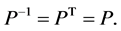
3)  can be written as:
  for a non-singular matrix
Definition 1.3 [29]. An  matrix
  is called diagonally dominant if

and strictly diagonally dominant if

The current paper is organized as follows. In Section 2, new algorithms for solving linear systems of equations of tridiagonal type via transformations are given. In Section 3, concluding remarks are given. MAPLE procedures are given in Section 4. Illustrative examples are presented in Section 5.
Throughout this paper, the word “simplify” means simplifying the expression under consideration to its simplest rational form.
2. Main Results
In this Section, we are going to consider the derivation of new algorithms for solving linear systems of equations of tridiagonal type (1) via transformations. For this purpose it is convenient to introduce three vectors 
 and
and  where
where
 (3)
(3)
By using the vectors c, y and z, together with the suitable elementary row operations (ERO’s), we see that the system (1) may be transformed to the equivalent linear system:
 (4)
(4)
The transformed system (4) is easy to solve by backward substitution. Consequently, the linear system (1) can be solved using the following algorithm:
The Algorithm 2.1, will be referred to as TRANSTRI-I algorithm. The cost of the algorithm is  multiplications/divisions and
  additions/subtractions.
Note that the algorithm TRANSTRI-I works properly only if  for all
At this point, it should be mentioned that if the coefficient matrix,  of the system (1) is positive definite or diagonally dominant, then the numeric algorithm TRANSTRI-I will never fail.
The following symbolic version algorithm is developed in order to remove the cases where the numeric algorithm TRANSTRI-I fails. The parameter “s” in the algorithm is just a symbolic name. It is a dummy argument and its actual value is zero.
The Algorithm 2.2, will be referred to as TRANSTRI-II algorithm.
In a similar manner, we may consider three vectors 
 and
and  where
where
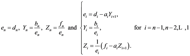 (5)
(5)
in order to develop a new algorithm.
We are going to focus on the symbolic version only. As in Algorithm 2.1, by using the vectors e, Y and Z, together with the suitable ERO’s, we see that the system (1) may be transformed to the equivalent linear system:
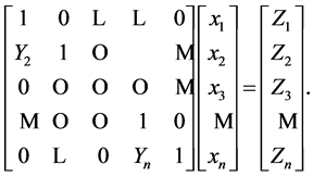 (6)
(6)
The transformed system (6) is easy to solve using forward substitution. Therefore the linear system (1) can be solved using the following algorithm:
The Algorithm 2.3, will be referred to as TRANSTRI-III algorithm.
Corollary 2.1. Let  be the backward matrix of the tridiagonal matrix
  in (2), and given by:
 (7)
(7)
Then the backward tridiagonal linear system
 (8)
(8)
has the solution:  where
where  is the floor function of k and
  is the solution vector of the linear system (1).
Proof. Consider the  permutation matrix
  defined by:
 (9)
(9)
For this matrix, we have:
 (10)
(10)
Since
 (11)
(11)
Then using (10) and (11), the result follows.
Corollary 2.2. The determinants of the coefficient matrices  and
and  in (2) and (7) are given respectively by:
 (12)
(12)
and
 (13)
(13)
where  and
and  satisfy (3) and (5).
3. Conclusions
There are many numeric algorithms in current use for solving linear systems of tridiagonal type. The Thomas algorithm is the well known numeric algorithm for solving such systems. However, all Thomas and Thomas-like numeric algorithms including the TRANSTRI-I algorithm of the current paper, fail to solve the tridiagonal linear system if  for any
  For example, all these numeric algorithms fail to solve the linear system:

since  although its coefficient matrix is invertible and its inverse is the following matrix

The symbolic algorithms TRANSTRI-II and TRANSTRI-III of the current paper are constructed in order to remove the cases where the numeric algorithms fail. These are the only symbolic algorithms for solving linear systems of tridiagonal type. Consequently, we are not going to compare them with numeric algorithms.
4. Computer Programs
In this Section, we are going to introduce MAPLE procedures for solving linear system of tridiagonal type (1). These procedures are based on the algorithms DETGTRI, TRANSTRI-II and TRANSTRI-III. The procedure of Program 1, alters the contents of the vectors 
 and
and  Eventually, the contents of the vectors
 and
and  are stored in
 and
and  respectively. The procedure of Program 2, alters the contents of the vectors
 and
and  Eventually, the contents of the vectors
 and
and  are stored in
 and
and  respectively.
5. Illustrative Examples
All results in this section are obtained by executing the MAPLE procedures of Program 1 and Program 2 presented in the previous section.
Example 5.1. Solve the tridiagonal linear system
 (14)
(14)
Solution: We have


and 
By applying the TRANSTRI-I algorithm, we get
• 
• 
• The solution vector is given by: .
.
Note that the coefficient matrix  in (14) is positive definite.
By applying the algorithms TRANSTRI-II and TRANSTRI-III, we obtain the same solution vector.
Example 5.2. Solve the tridiagonal linear system

Solution: Here, we have


 and
and 
By applying the TRANSTRI-I algorithm, we get
• 
• 
• The solution vector is given by: .
.
By using the algorithms TRANSTRI-II and TRANSTRI-III, we obtain the same solution vector.
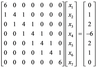
Example 5.3. Solve the tridiagonal linear system
 (15)
(15)
Solution: Here, we have


 and
and 
The numeric algorithm TRANSTRI-I fails to solve the linear system (15) since  Applying the TRANSTRI-II algorithm, it gives:
• 
• 
• The solution vector is given by:

Using the TRANSTRI-III algorithm, it gives the same solution vector.
Acknowledgements
The authors wish to thank anonymous referees and the editorial board for useful comments that enhanced the quality of this paper.