Simulation of a DI Diesel Engine Performance Fuelled on Biodiesel Using a Semi-Empirical 0D Model ()
1. Introduction
Reaching lower toxicity of exhaust gases, whilst reducing fuel consumption is one of the modern trends in automobile engineering research. The characteristics of fuel play an important role in the performances of the engine. Gasoil has been for years the main fuel for diesel engine but, due to the reducing availability of fossil energy resources and the stricter rules on engine emission [1], and researchers have been investigating the use of alternative fuels. Biodiesel, which is obtained through transesterification process of vegetable oil, has been proven to be a high potential substitute for conventional gasoil [1-3].
Simulation and mathematical modeling of diesel engine are scientific topics carried out by several research works. Nowadays, there mainly exist three types of approaches for diesel engine simulation: 0 dimensional thermodynamic, quasi dimensional and multi dimensional (Computational Fluid Dynamic). A well documented discussion on these models can be found in [4].
Many commercial computer codes based on computational fluid dynamic (CFD) [5] provide useful tools to simulate in diesel engine processes. CFD permits simulating real engine conditions with the aim of understanding how physical and chemical conditions will affect engine performances. One of the main disadvantages of CFD tools is that they are too slow to be implemented in car vehicles control software and their use as optimization or simulation tools which have a very high computer cost. Car control software mostly uses semi empirical 0D model due to their simplify approach, their quickness of implementation inside the electronic unit control of the engine. For engine simulation and optimization, several commercial codes using semi empirical models exist [6, 7]. The cost for license acquisition and the access to source codes are some of the limitations of this software in term of scientific research. To get away from these limitations we used an open source numerical calculation software called Scilab [8] in which we implemented our model.
The model we implemented in our study is based on the engine performance Wiebe model [9]. It has been for years used in diesel engine simulation, and it requires adjustable experimental coefficients related to engine specification. Since the scope of the work is about defining effect of biodiesel on engine performances, the experimental coefficient can be considered constant since they don’t depend on the fuel used.
One of the limitations of the Wiebe model is that it doesn’t predict well the combustion during the premix phase of combustion. That limitation is overcome by Watson model of heat release in diesel engine [4,10]. Both Wiebe and Watson model don’t take into account the ignition delay of the injected fuel in the cylinder, thus obliging us to find a suitable relationship to predict ignition delay. Pischinger et al. [11] defined a correlation between the length of the fuel spray at which ignition occurs and the temperature and pressure at the start of injection angle. Others strong relationship between ignition delay and start of injection angle was experimentally derived by Razlejtsev [12] and Lechivskii [13]. In these relationships, the ignition delay is described using an Arrenhius correlation between the pressure and temperature at start of injection angle and activation energy of the fuel. However, these relationships don’t give a methodology to compute ignition delay for other types of fuels such as biodiesel. Most of the coefficients used in these relationships refer to experiments conducted in engine running under conventional diesel, thus leading one to the search of suited relationship which can take into account certain physical and chemical specificities of fuel used.
The present work, describes a semi empirical model used to predict how performances parameters such as thermal efficiency, specific fuel consumption, indicative pressure and indicative pressure will vary depending type of fuel used. The model is developed Fuel for diesel engine control purpose when running on biodiesel. Spray behavior of biodiesel is not covered in this work but some useful computational studies about the topic can be found in [14,15], and it will be inserted in further development of the model.
2. Governing Equations
The model used in the present study is a semi-empirical model, based on the work of I. I. Wiebe [1] and the heat release calculation model of Watson [2] and the work of Grondin [3], figure 1 shows a flow chart description of the model, where one can see the input information needed as well as the output data obtained from the model. The next section presents the main governing equations of the model as well as the constant used for our calculations. The model was implemented using an open source calculation code for rapid treatment of the information.
2.1. Ignition Delay Model
The initial Wiebe model was not taking into account the ignition delay period when calculating the combustion process. Wiebe model computes the heat release starting from the injection start angle, whereas it has been shown that ignition occurs after a certain amount of time after injection (ignition delay), due to complex chemistry processes.
In our model we used the model proposed by Hardenberg and Haze [4] which takes into account one of the main properties of the fuel which is believed to influence the delay period as in the cetane number.
 ,
,

Figure 1. Model algorithm; CN—Cetane number; CC— Chemical composition; P—Power; FC—Fuel consumption; LHV—Lower heating value.
where UP is the mean piston speed in m/s; R is the gas constant in J/kmol-K; ε is the compression ratio of the engine; CN is the cetane number of the fuel Pim and Tim are the pressure in bar and temperature in Kelvin at the intake manifold; nc is the polytropic exponent for compression.
2.2. Step by Step Computation
The next step of the model is the fuel engine cycle model; here we determine the pressure inside the cylinder at any angle of rotation of the crankshaft taking into account the start of injection angle the duration of combustion and other parameters. As a result one will be able to determine the different parameters characterizing the efficiency of work of the engine, such as the specific consumption, the effective power and efficiency. The model computes the full process taking place inside the cylinder, with the calculations being made for each stroke of engine cycle.
2.3. Admission Stroke
The pressure of the working medium at the end of the admission stroke is given in Pascal by
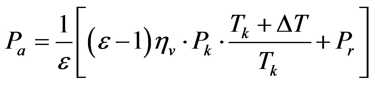 ,
,
where ηυ is the admission coefficient, Pk is the pressure at inlet valves in MPa, Tk the temperature at inlet valves in K, ΔT is the temperature gradient due to the heating of engine elements in MPa, Pr is the residual gases pressure in MPa.
The temperature of the working medium at the end of the admission stroke is given in Kelvin by
 ,
,
where Tk is the temperature of residual gases in K, ς is the coefficient of residual gases.
The theoretically necessary (stoichiometric) quantity of air for the combustion of 1 kg of fuel is given as , its value is dependent of the chemical composition of the fuel used and is determined by
 ,
,
where, C, H and O are respectively, the ratio of carbon, hydrogen and oxygen in the fuel chemical composition.
The specific volume of the working medium at the end of the admission stroke is given in m3/kg by
 ,
,
where μair is the molecular mass of air.
2.4. Compression Stroke
The parameters of the working medium during the compression stroke are computed using the polytropic process equation.
The pressure at a given time is given in MPa by

where ν is the current value of specific volume defined as
 ,
,
σ is the kinematic function of the motion of the piston
 ,
,
where λ is the ratio of the lengths of the crankshaft and the connecting rod, φ is the current angle of rotation of the crankshaft.
The specific work of compression is then determined in MJ/Kg by

2.5. Power Stroke
2.5.1. Heat Release Model
The admission, compression and ignition delay phase being computed, the next is step of the model is the heat release calculation. Our heat release model computes two phases of the combustion process, the premixed and diffusion phase.
The current fraction of fuel burnt —where φ is the current crankshaft position angle—is computed using a double Wiebe function [2], we then have
 ,
,
with xp and xd representing the fraction of fuel burnt in each phase of the combustion process, β representing the fraction of fuel injected during the premixed phase.
For each phase of the combustion phase (equation 10) we can write
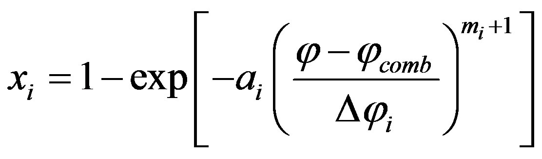 ,
,
where ai and mi are experimental shaping coefficient of the Wiebe function; φcomb is the start of ignition angle;  is the combustion duration for each phase.
The normalized combustion rate (1/deg) is computed by derivation of xi about φ.
2.5.2. Combustion Model
The combustion effectiveness which accounts for heat loss (heat loss due to heat transfer to the walls, hydraulic losses due to the flow of gases) ratio is first defined by

where δ is a heat release factor which takes into account the ration of unburned fuel; ψ—is a ratio of used heat.
The total specific heat of combustion used (instantaneous heat release) is given in MJ/Kg by
 ,
,
where Hu is the net calorific value of the used fuel in MJ/Kg and α is the coefficient of excess air and γ is the ratio of specific heat during the combustion process, according to [16] is value can be taken as constant going from 1.3 to 1.35.
Pressure calculation at any moment of the power stroke is computed using the first law of thermodynamic and can described for the evolution of the pressure/volume indicator diagram from a point 1 to 2 by
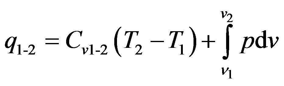 ,
,
where: q1-2 specific heat used to increase the internal energy from point 1 to 2 in the diagram; Cv1-2 is the average specific heat the working medium for constant pressure from point 1 to 2.
Assuming each volume step is small enough and using the trapezoidal method to simplify the integral in formula (14) and expressing Cv1-2 in term of P2 using the Mayer’s formula, we determine the value of the pressure at any given time of the power stroke using the simplified equation
 ,
,
Δx1-2 is the ratio of fuel burnt from point 1 to 2.
Specific work of gases during the combustion stroke is given in MJ/Kg by
 .
.
Further description of the model can be found in [9], here we presented the main equations for combustion that will have a greater impact on the engine performance calculation.
3. Results and Discussion
3.1. Model Validation
The validation of the model consisted in comparing experimental results from previous researches with simulation results using the model. For this purpose, experimental data obtained by Sahoo et al. [17] from a single cylinder diesel at rated speed were compared with the model simulation. To further investigate the validity of the model we proceeded to the simulation of a six cylinder direct injection diesel at different crankshaft rotational speed, results were compared with experimental data obtained by Ahmet et al. [18].
The simulation were performed on a 3 Go of RAM Dual core computer with a time step of 0.1 crank angle degrees, a full simulation took about 6 minutes to complete. The parameters of the model were adjusted to closely match the experimental results. The diffusive combustion duration was estimated about 75 and 60 degrees of rotation of the crankshaft for the first and second experiment respectively using least square fitting technique.
3.1.1. Experimental Setup
Tables 1 and 2 present the engines specifications for each experiment. The default injection timing for the second experiment was determined from the fuel line pressure diagram. The second experiment was performed under varying crankshaft rotational speed—1000, 1250, 1500, 1750 and 2000 rpm.
The calorific value of the diesel fuel was also modified for the second experiment to 42.5 MJ/kg to match experimental input data, remaining properties of the fuel were kept unchanged. To perform comparison we used fuel characteristics that were stated in the work of Sahoo et al. [17], but due to the lack of some relevant information that shall be given as entry parameters to our model we had to add them according to diesel fuel standards. Specifications of the validating fuel can be seen at table 3.
3.1.2. Comparison of Experimental result with Simulation
Figure 2 shows the in cylinder pressure during the combustion phase for experiment number 1. It can be seen that the simulated curve has a similar shape with the experimental curve, the peak pressure, starting and ending pressure values are almost the same. The slight gap between the curves can be due to the fact that the ignition delay model underestimated the experimental ignition delay obtained.
Table 4 shows comparison of simulation results to experimental performances results. It can be seen than the peak pressure is estimated with good accuracy by the model. However the occurrence of the peak pressure is about six degrees earlier in the simulated result, this is an issue that should investigated in further researches. The break power is estimated with an accuracy of 95%,