Computing Approximation GCD of Several Polynomials by Structured Total Least Norm ()
1. Introduction
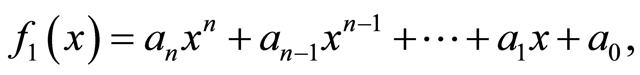
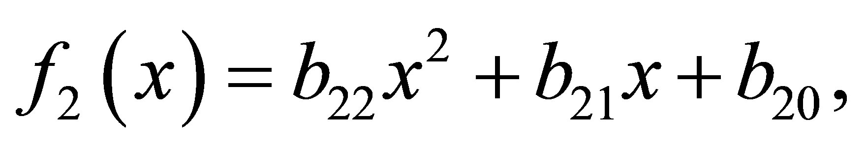
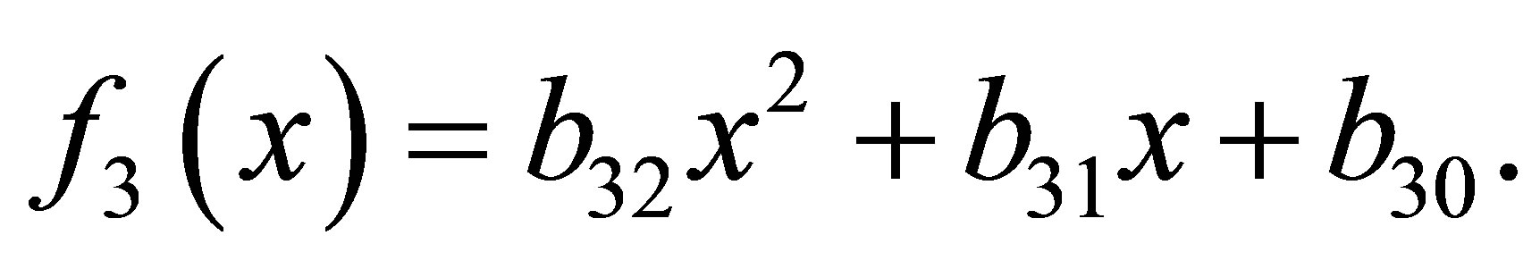
Let  be the degree of
  and
and  be the set of univariate polynomials.
  stands for the spectral norm of the matrix
 .
.  and
and  are the vector spaces of complex
  vectors and
  matrices, respectively. Transpose matrices and vectors are denoted by
  and
and .
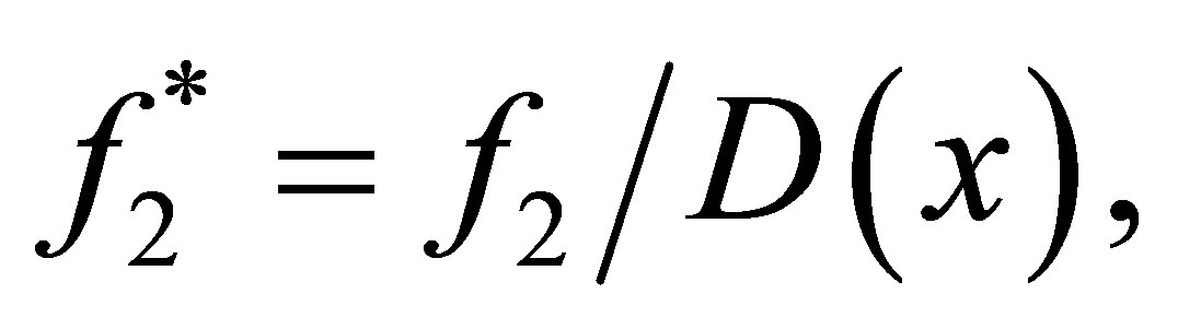
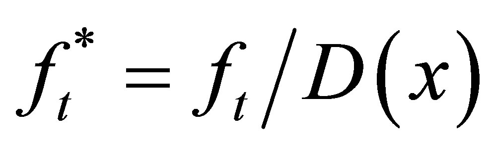
.  denotes the greatest common divisor for the polynomials
  and
and . We use
  to stand for the rank of matrix
 .
.
In this paper, we consider the following problem. Let 

 , namely

Problem 1.1. Set  be a positive integer with
 . We wish to compute


 such that


and
is minimized.
The problem of computing approximate GCD of several polynomials is widely applied in speech encoding and filter design [1], computer algebra [2] and signal processing [3] and has been studied in [4-7] in recent years. Several methods to the problem have been presented. The generally-used computational method is based on the truncated singular decomposition (TSVD) [8] which may not be appropriate when a matrix has a special structure since they do not preserve the special structure (for example, Sylvester matrix). Another common method based on QR decomposition [9,10] may suffer from loss of accuracy when it is applied to ill-conditioned problems and the algorithm derived in [11] can produce a more accurate result for ill-conditioned problems. Cadzow algorithm [12] is also a popular method to solve this problem which has been rediscovered in the literature [13].
Somehow it only finds a structured low rank matrix that is nearby a given target matrix but certainly is not the closet even in the local sense. Another method is based on alternating projection algorithm [14]. Although the algorithm can be applied to any low rank and any linear structure, the speed may be very slow. Some other methods have been proposed such as the ERES method [15], STLS method [16] and the matrix pencil method [17]. An approach to be described is called Structured Total Least Norm (STLN) which has been described for Hankel structure low rank approximation [18,19] and Sylvester structure low rank approximation with two polynomials [20]. STLN is a problem formulation for obtaining an approximate solution  to an overdetermined linear system
  preserving the given structure in
  or
or .
.
In this paper, we apply the algorithm to compute the structured preserving rank reduction of Sylvester matrix. We introduce some notations and discuss the relationship between the GCD problems and low rank approximation of Sylvester matrices in Section 2. Based on STLN method, we describe the algorithm to solve Problem 1.1 in Section 3. In Section 4, we use some examples to illustrate the method is feasible.
2. Main Results
First of all, we shall prove that Problem 1.1 always has a solution.
Theorem 2.1. Suppose that 


 ,
, 

 and
and  are defined as those in Problem 1.1. There exist
 ,
,  with
with ,
,  and
and
 such that for all
 ,
,  with
with ,
,  and
and

 .
.
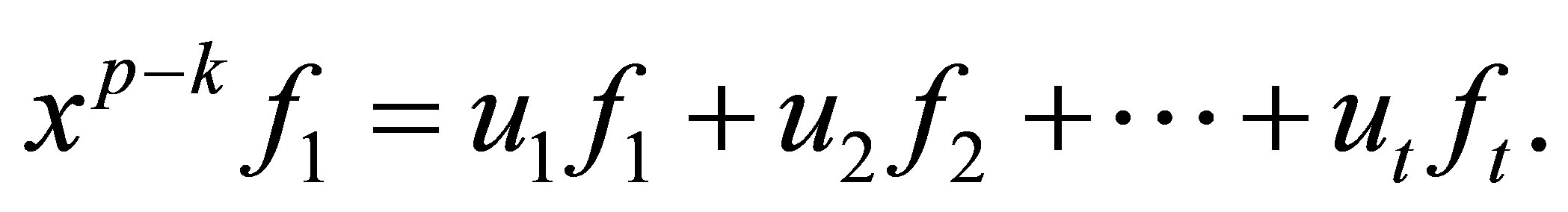
We have

Proof. Let  be monic with
  and set
  with
with . For the real and imaginary parts of the coefficients of
  and of
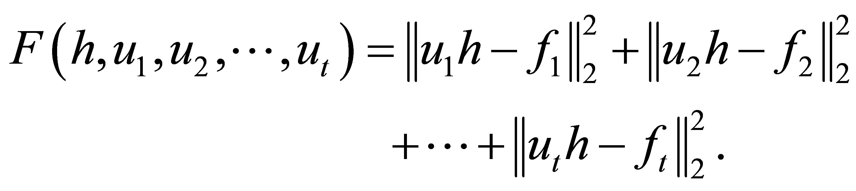
 . We are considered with the continuous objective function
We will prove that the function has a value on a closed and bounded set of its real argument vector which is smaller than elsewhere. Consider  and
and  with a GCD of degree
  for
for . Clearly, any
  and
and  with
with

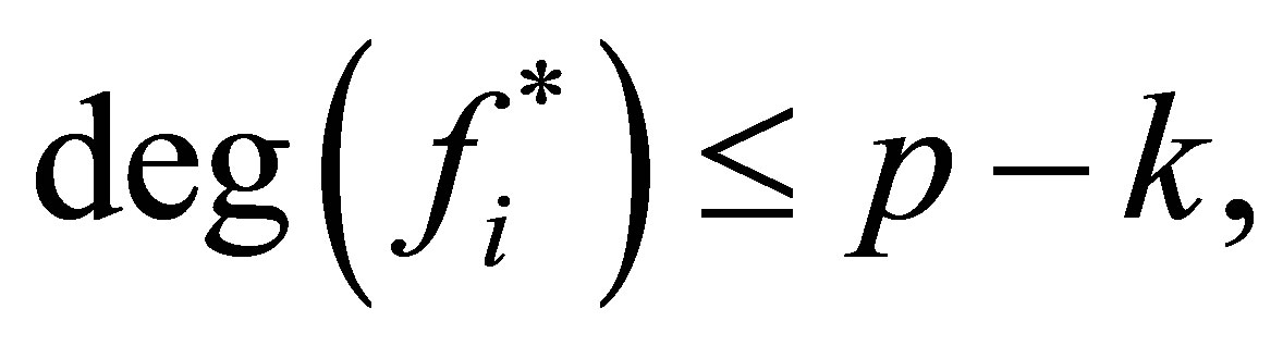
can be discarded. So from above,we know that the coefficients of 

 can be bounded and so can the coefficients of


 by any polynomials factor coefficient bound. Thus the function’s domain
  is restricted to a sufficiently large ball. It remains to exclude
 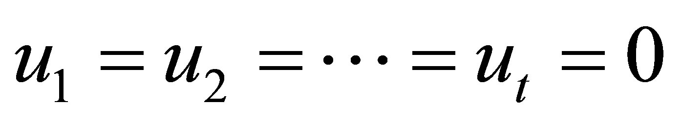 as the minimal solution. We have
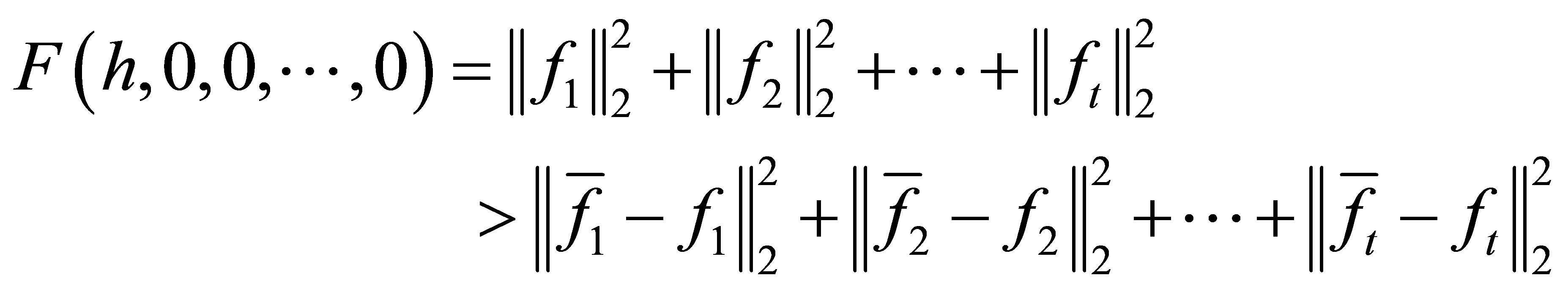 .
.
In conclusion, the theorem is true.
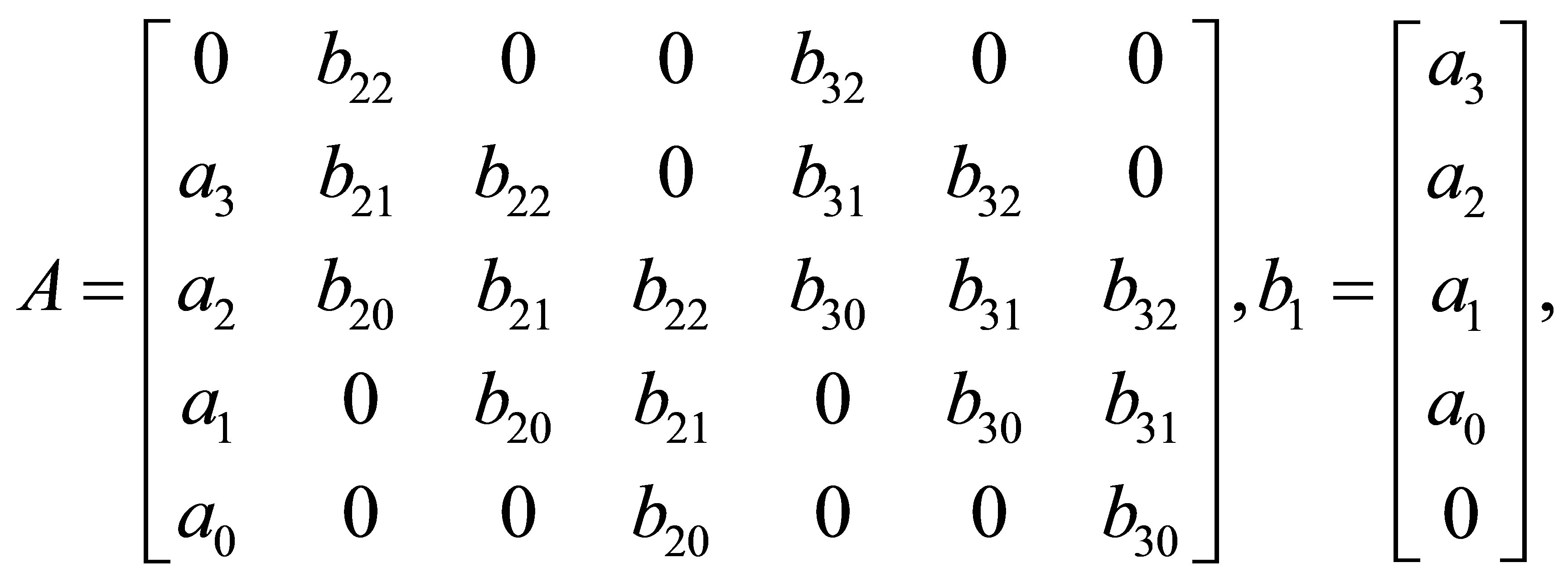
Now we begin to solve Problem 1.1, we first define a  matrix associated with
  as follows

and an  matrix associated with
 as
as
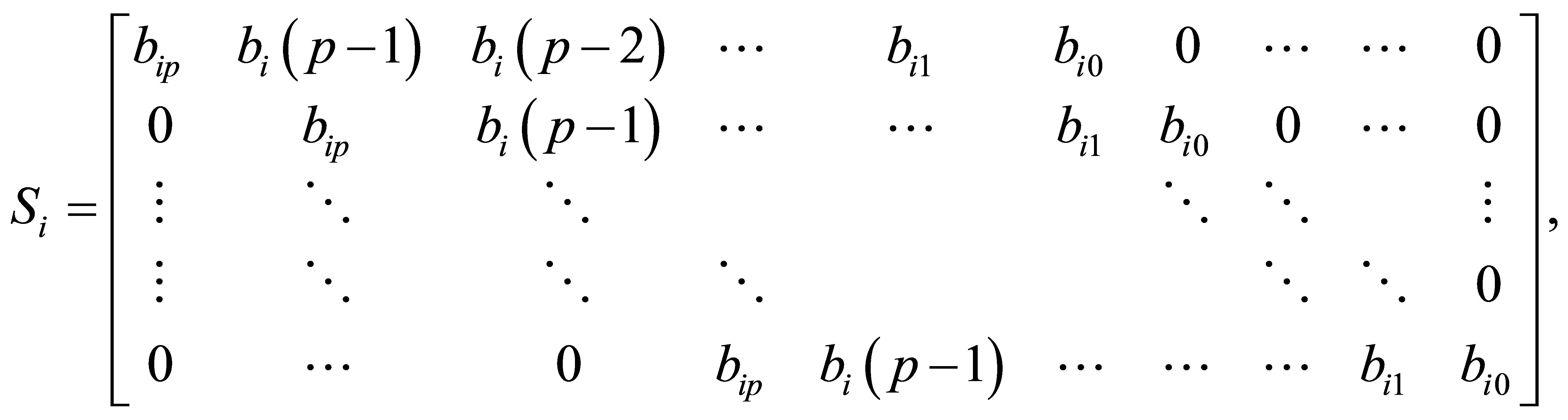
An extended Sylvester matrix or a generalized resultant is then defined by

Deleting the last  rows of
  and the last
  columns of coefficients of
  separately is
 , We get the
  -th Sylvester matrix
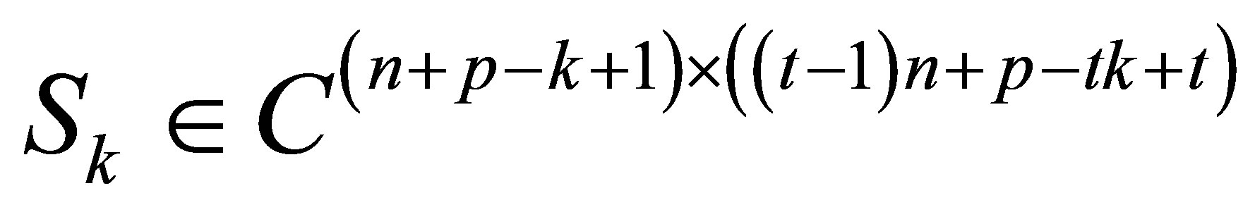

It is well-known that 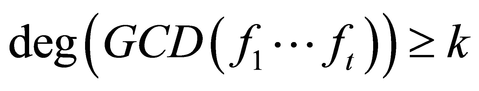 if and only if
  has rank deficiency at least 1. We have

(2.1)
where  is the
  -th Sylvester matrix generated by

 .
.
From above, we know that (2.1) can be transformed to the low rank approximation of a Sylvester matrix.
If we use STLN [16] to solve the following overdetermined system
for , where
  is the first column of
  and
and  are the remainder columns of
 , then we get a minimal perturbation
  of Sylvester structure satisfying

So the solution with Sylvester structure is 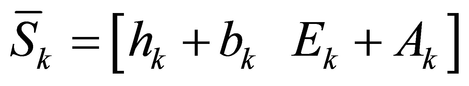 and
and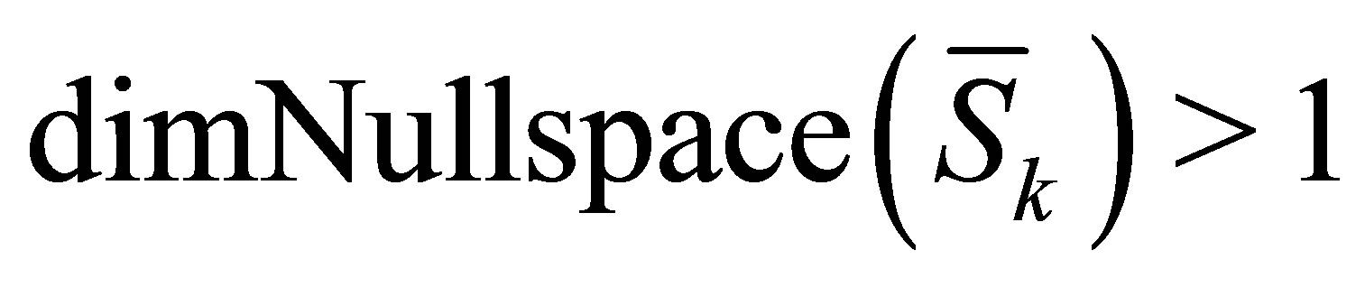 .
.
We will give the following example and theorem to explain why we choose the first column to form the overdetermined system.
Example 2.1. Suppose three polynomials are given

The matrix  is the Sylvester matrix generated by

 and
and 
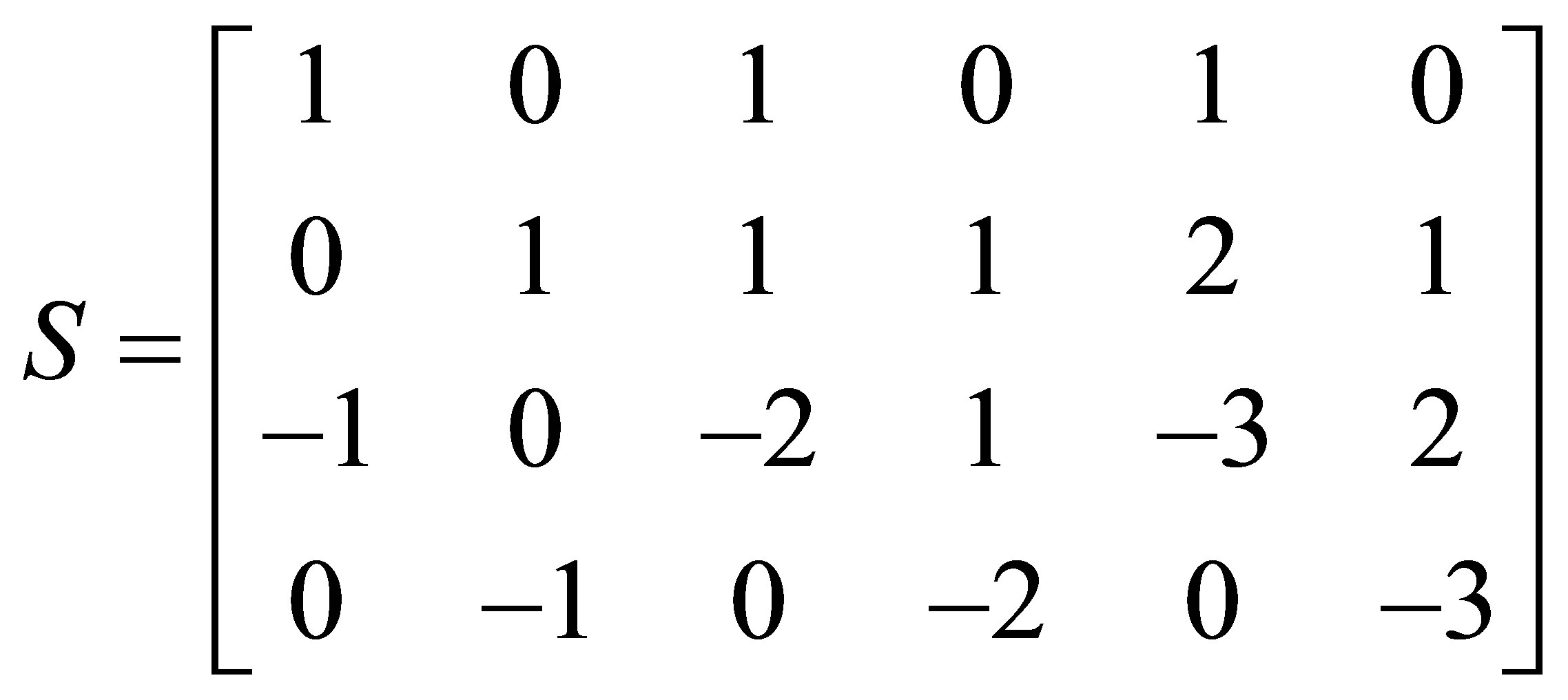
The matrix  is partitioned as
 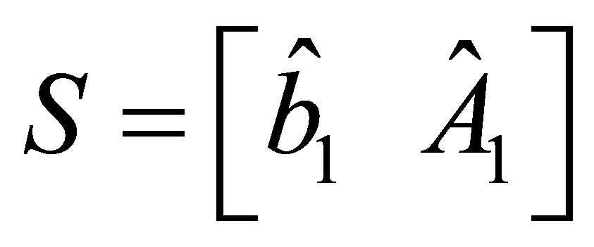 or
or , where
  is the first column of
 , whereas
 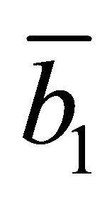 is the last column of
 .
.
The overdetermined system
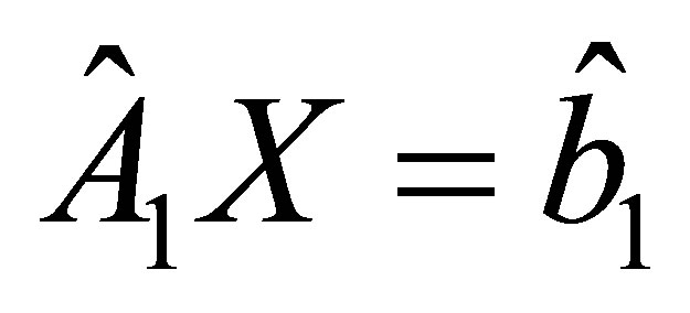
has a solution , while the system
has no solution.
Theorem 2.2. Suppose that 

 ,
, 


 and
and  are defined as those in Problem 1.1 and
  is the
  -th Sylvester matrix of

 . Then the following statements are equivalent.
1) ;
;
2)  has a solution, where
  is the first column of
  and
and  are the remainder columns of
 .
.
Proof.  Suppose
  has a nonzero solution, then
 . Since
  is the first column of
 , obviously, the dimension of the rank deficiency of
  is at least 1.
 Suppose the rank deficiency of
 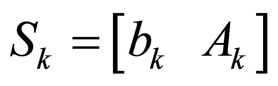 is at least 1 and
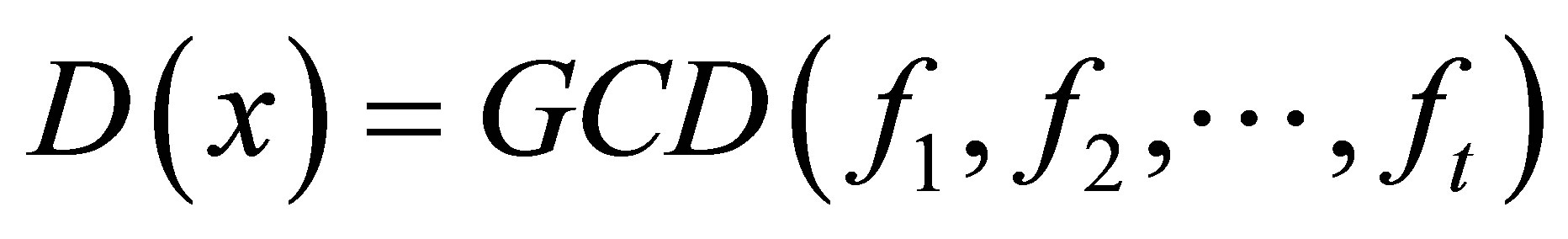 ,
, 

 . Multiplying the vector
  to the matrix
 , then we obtain
 (2.2)
(2.2)
Next we will prove that  has a solution. If we multiply the vector
  to two sides of the equation
 , it turns out to be
 (2.3)
(2.3)
The solution  of equation (2.3) is equal to the coefficients of polynomials

 such that
We can get  and
and 
 from
from  . Dividing
  by
by , we obtain a quotient
  and a remainder
  satisfy
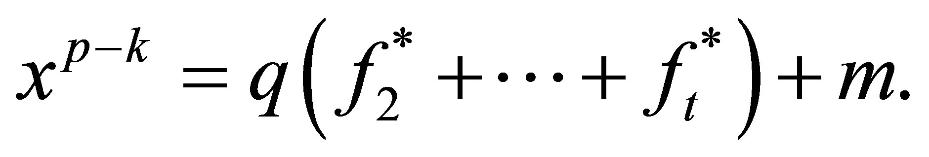
where 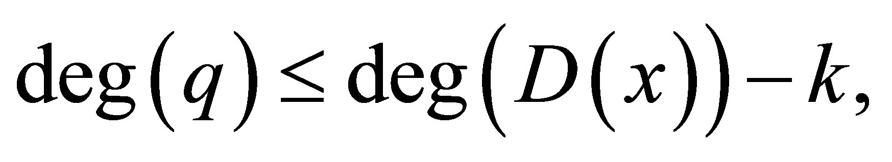
 . Now we can get that

are solutions of Equation (2.3), since

and

Next, we will illustrate for any given Sylvester matrixas long as all the elements are allowed to be perturbed, we can always find  -Sylvester structure matrices
  satisfy
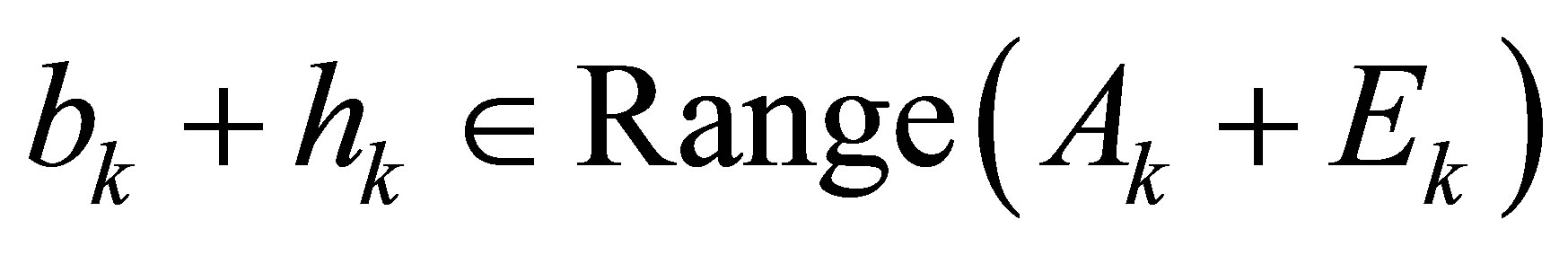 , where
  is the first column of
  and
and  are the remainder column of
 .
.
Theorem 2.3. Given the positive integer , there exists a Sylvester matrix
  with rank deficiency k.
Proof. We can always find polynomials  with
with ,
,  and
and . Hence
  is the Sylvester matrix of
  and its rank deficiency is k.
Corollary 2.1. Given the positive integer , and
, and  -th Sylvester matrix
 , where
  ,
,  , it is always possible to find a
  -th Sylvester structure perturbation
 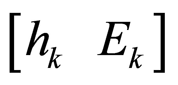 such that
 .
.
3. STLN for Overdetermined System with Sylvester Structure
In this section, we will use STLN method to solve the overdetermined system

According to theorem 2.3 and corollary 2.1, we can always find Sylvester structure  with
with  . Next we will use STLN method to find the minimum solution.
First, we define the Sylvester structure preserving perturbation  of
of 

can be represented by a vector
 .
.
We can define a matrix  such that
 .
.

where  is a
is a  identity matrix.
We will solve the equality-constrained least squares problem
 (3.1)
(3.1)
where the structured residual  is
is
By using the penalty method, the formulation (3.1) can be transformed into
 (3.2)
(3.2)
where  is a large penalty value.
Let  and
and  stand for a small change in
  and
and , respectively and
  be the corresponding change in
 . Then the first order approximate to
  is
is
Introducing a matrix of Sylvester structure  and
and

(3.2) can be approximated by
 (3.3)
(3.3)
where  satisfies that
 (3.4)
(3.4)
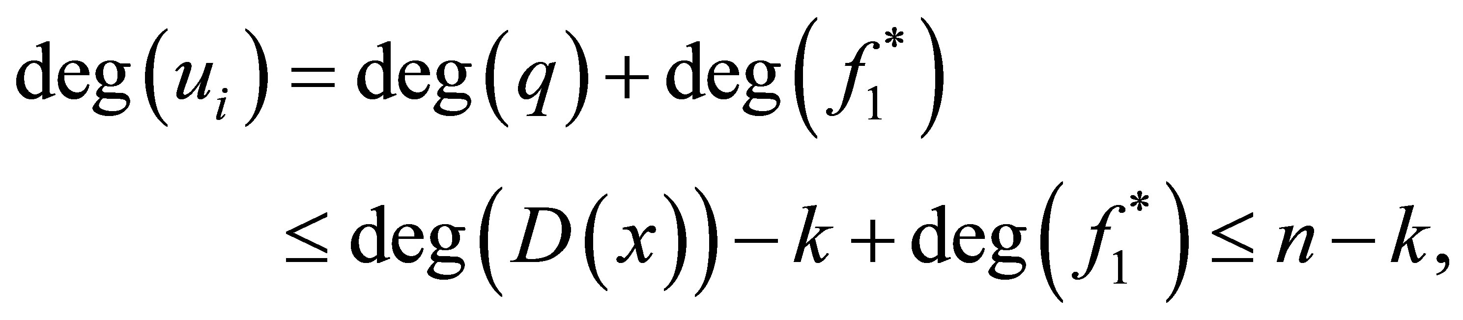
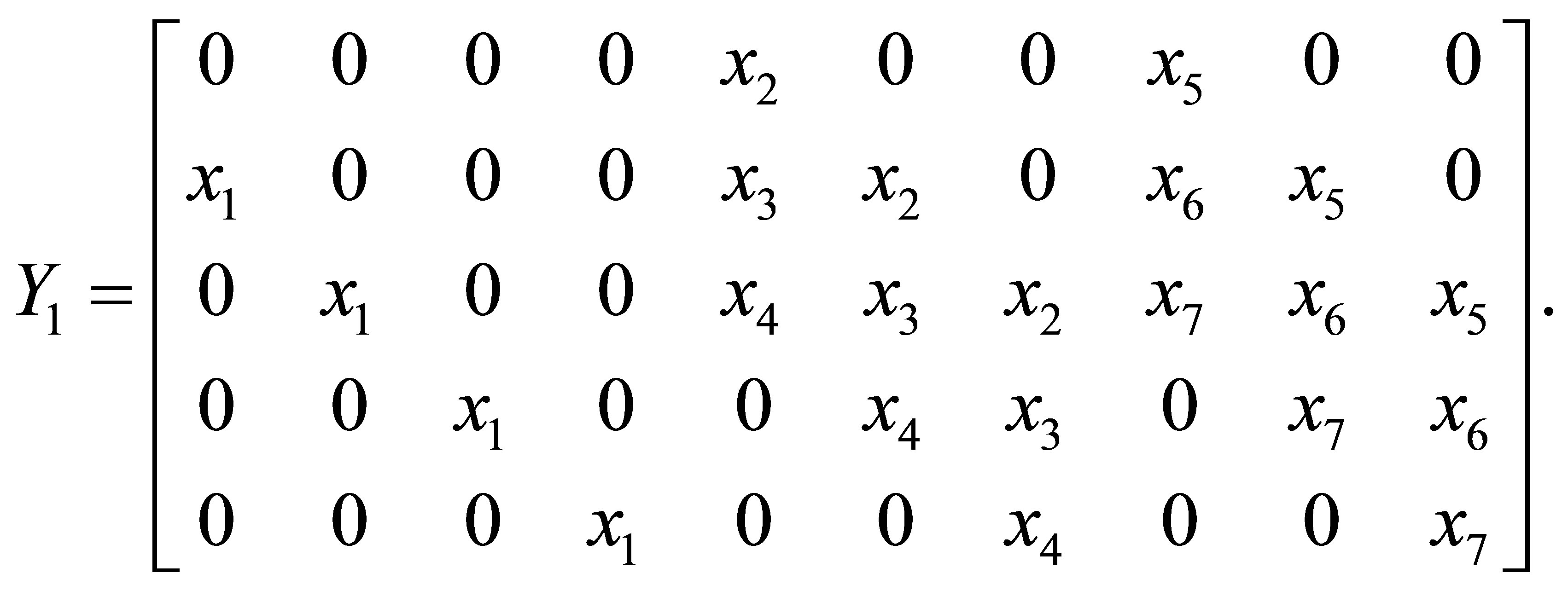
In the following, we present a method to obtain the matrix . Suppose


 and
and  are defined as above. Multiplying the vector

to the two sides of equation (3.4), it becomes

Let , we obtain
 (3.5)
(3.5)
where  is the polynomial with degree
  which is generated by the subvector of
 :
:
 is the polynomial with degree
  which is generated by the subvector of
 :
:

 is the polynomial with degree
  which is generated by the subvector of
 :
:

 is the polynomial with degree
  which is generated by the subvector of
 :
:
 is the polynomial with degree
  which is generated by the subvector of
 :
:

 is the polynomial with degree
  which is generated by the subvector of
 :
:

Here we will present a simple example to illustrate how to find .
.
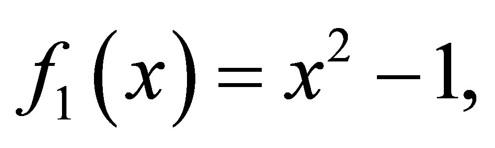
Example 3.1. Suppose ,
,  and
and 
then
4. Approximate GCD Algorithm and Experiments
The following algorithm is designed to solve Problem 1.1.
Algorithm 4.1.
Input-A Sylvester matrix S generated by 


 , respectively, an integer
  and a tolerance
 .
.
Output-Polynomials 


 and the Euclidean distance
 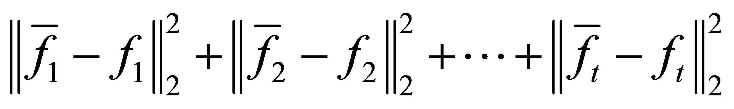 is to a minimum.
1) Form the  -th Sylvester matrix
  as the above section, set the first column of
  as
as  and the remainder columns of
  as
as . Let
. Let .
.
2) Calculate  from
from 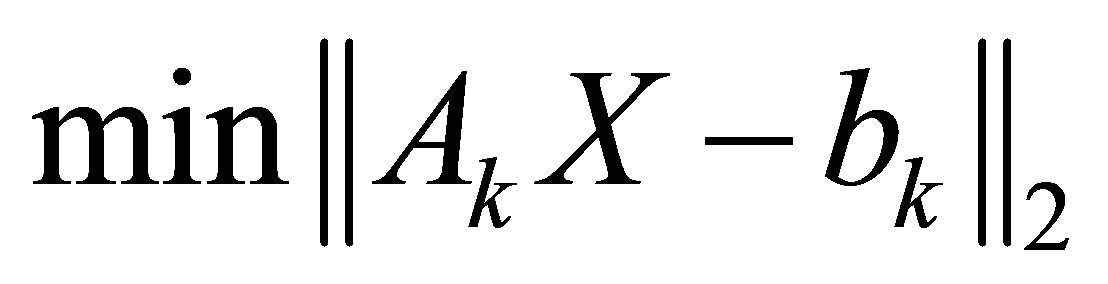 and
and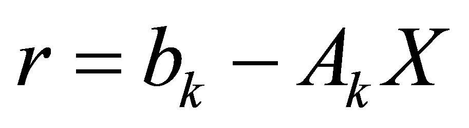 . Compute
  and
and  as the above section.
3) Repeat
(1) 
(2) Let 
(3) Form the matrix  and
and  from
from , and
, and  from
from . Let
. Let 

 until
until  and
and 
4) Output the polynomials 


 constructed from
Given a tolerance , we can use the Algorithm 4.1 to compute an approximate GCD of
 . The method begin with
  using Algorithm 4.1 to compute the minimum perturbation
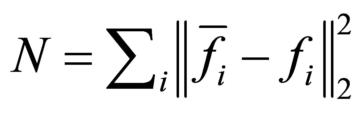
with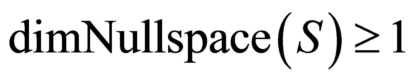 . If
. If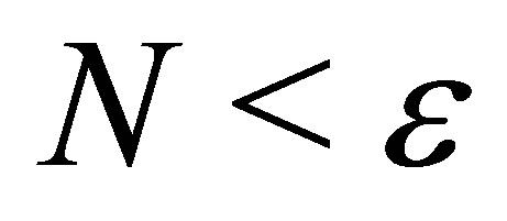 , then we can compute the approximate GCD form matrix
 . Otherwise, we reduce
  by one and repeat the Algorithm 4.1.
Example 4.1. We wish to find the minimal polynomial perturbations  and
and  of
of
satisfy that the polynomials  and
and  have a common root. We take two cases into account.
Case 1: The leading coefficients can be perturbed. Let  and
and , after 3 iterations, we get the polynomials
  and
and 


with a minimum distance

Case 2: The leading coefficients can be perturbed. Let  and
and , after 3 iterations, we have the polynomials
  and
and :
:

with a minimum distance

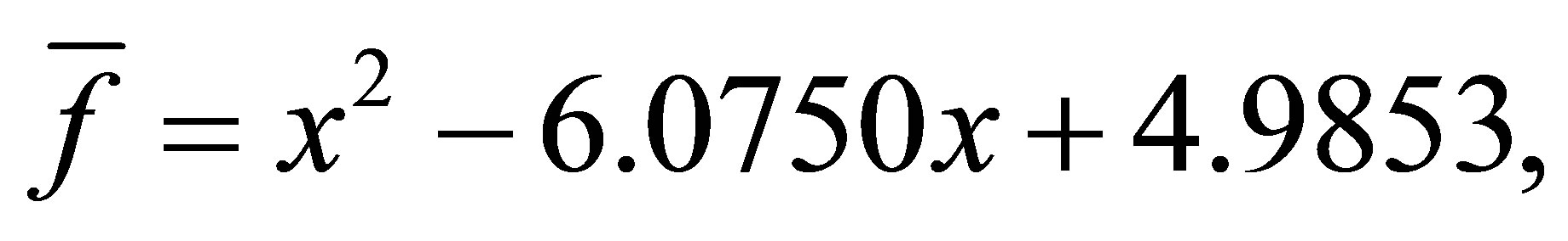
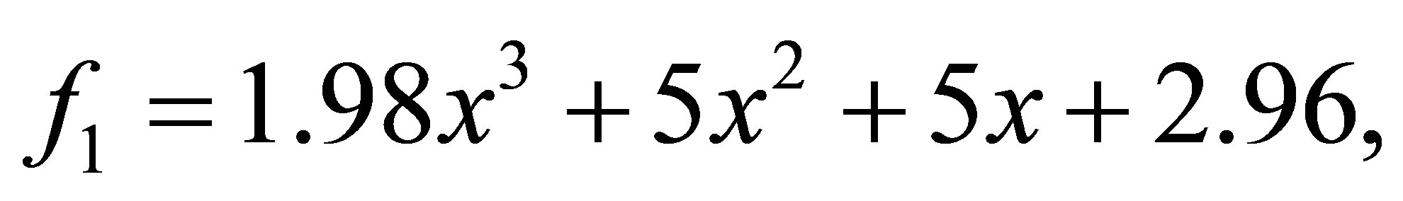
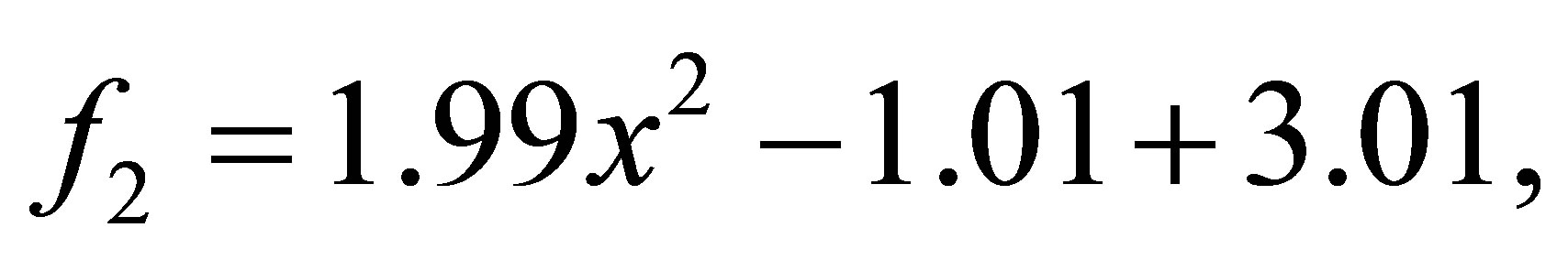
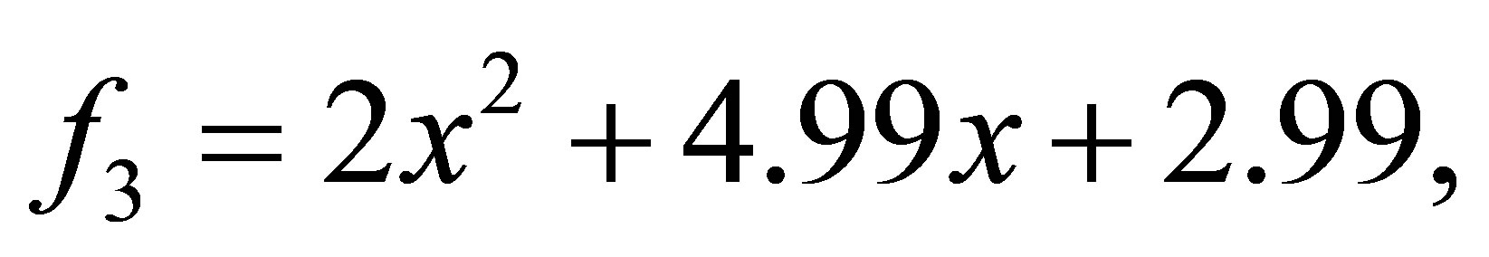
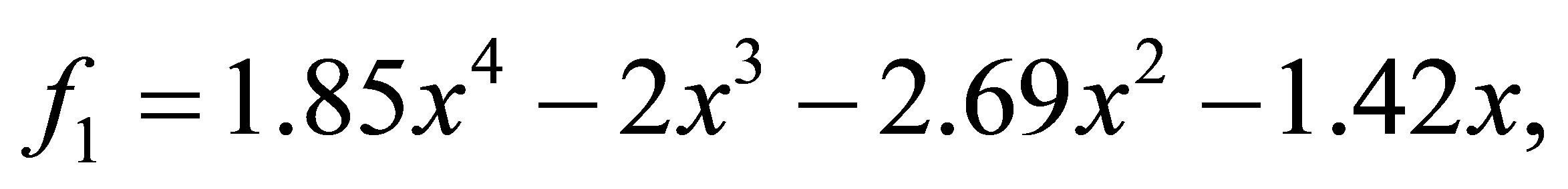
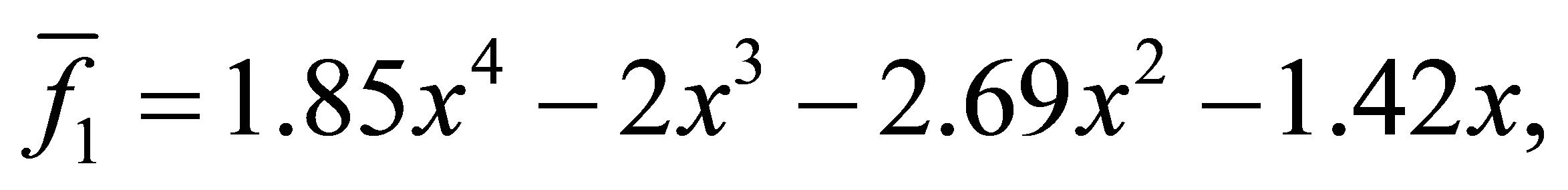
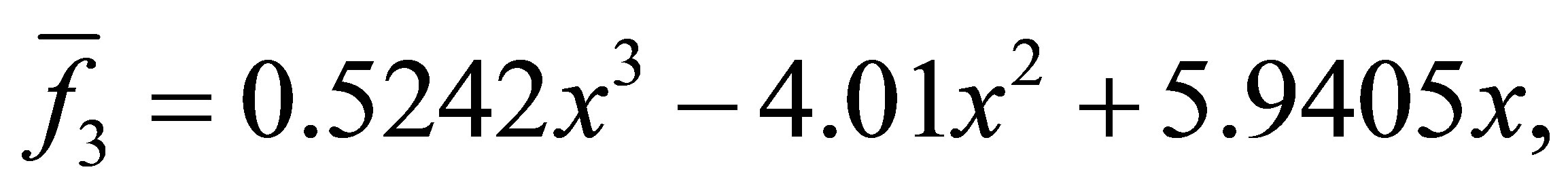
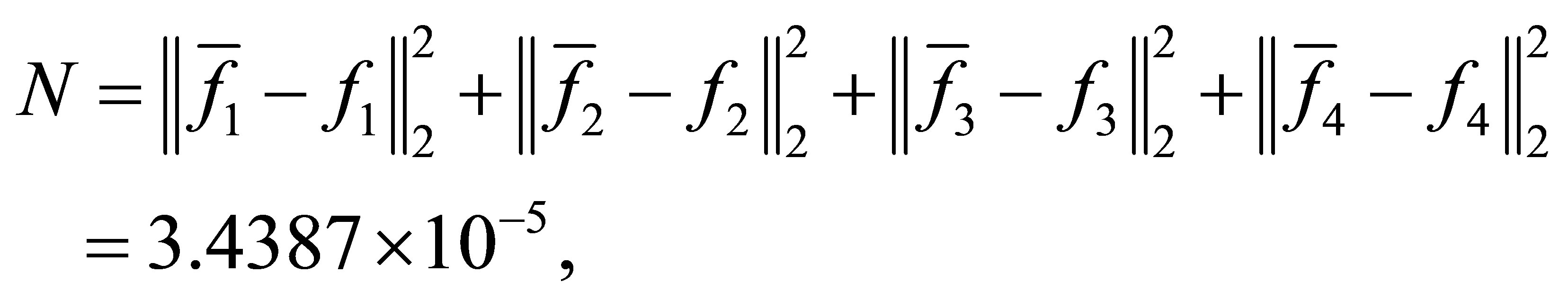
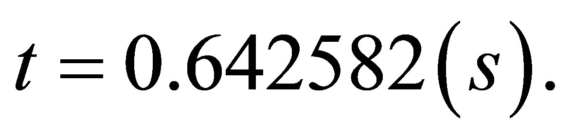
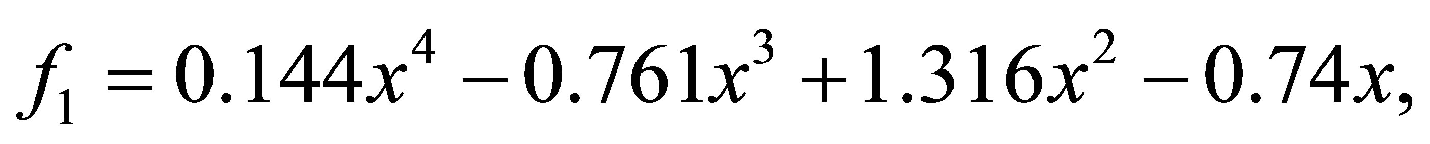
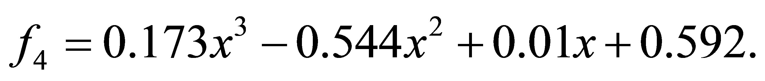
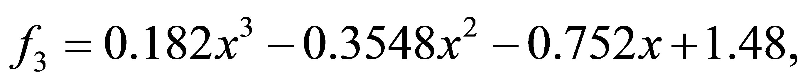
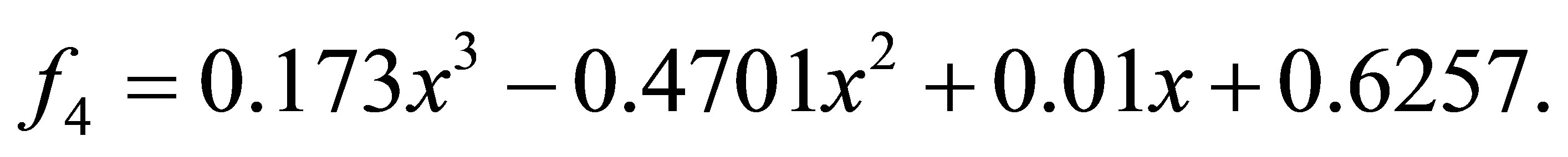
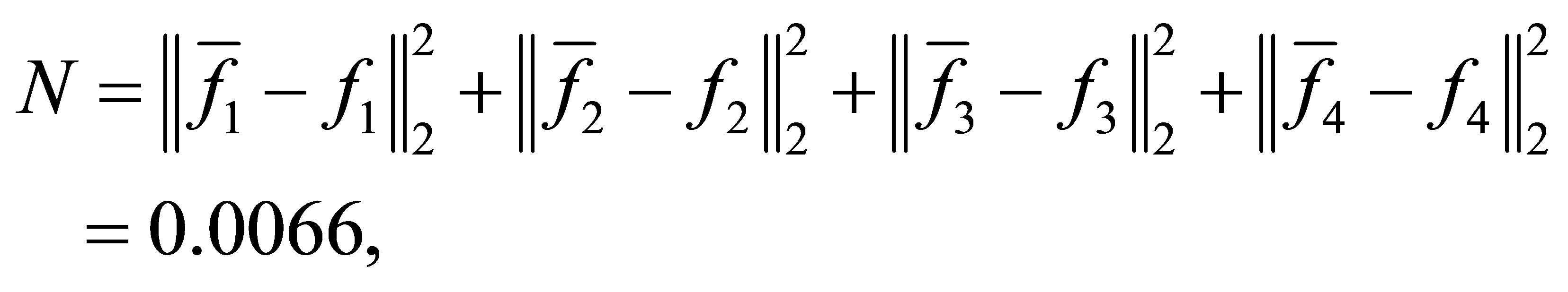
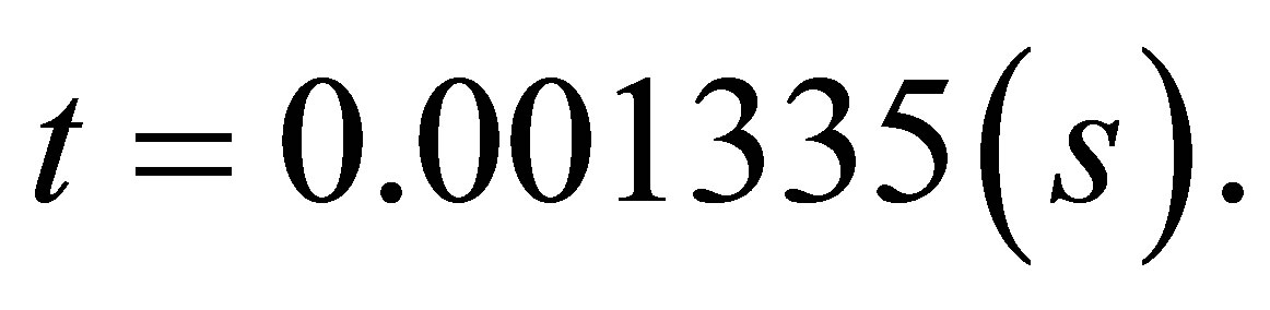
Example 4.2. Let ,
,  and
and
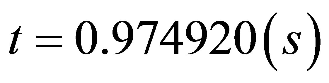
after 8 iterations, we have the polynomials


with a minimum distance

and the CPU time
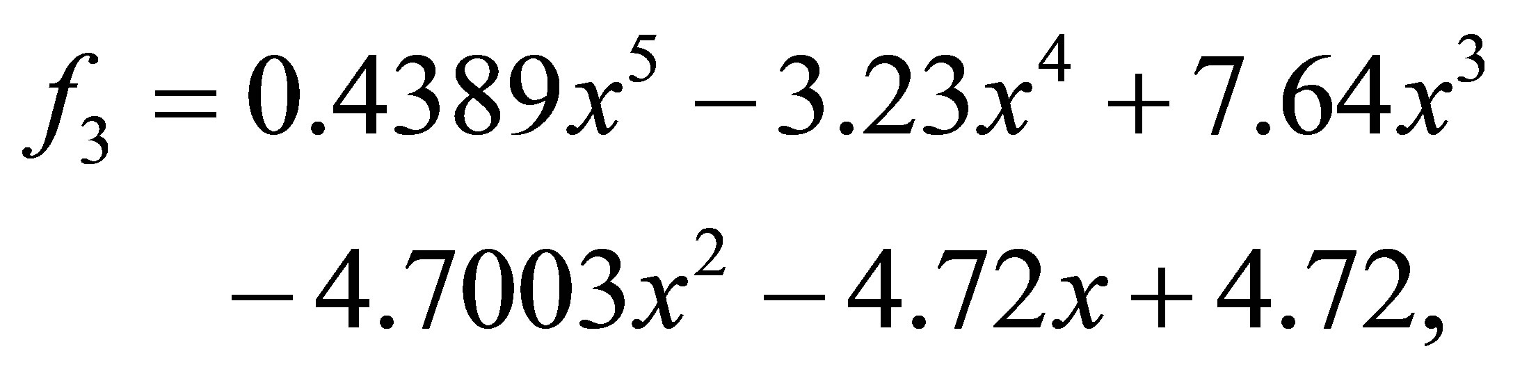
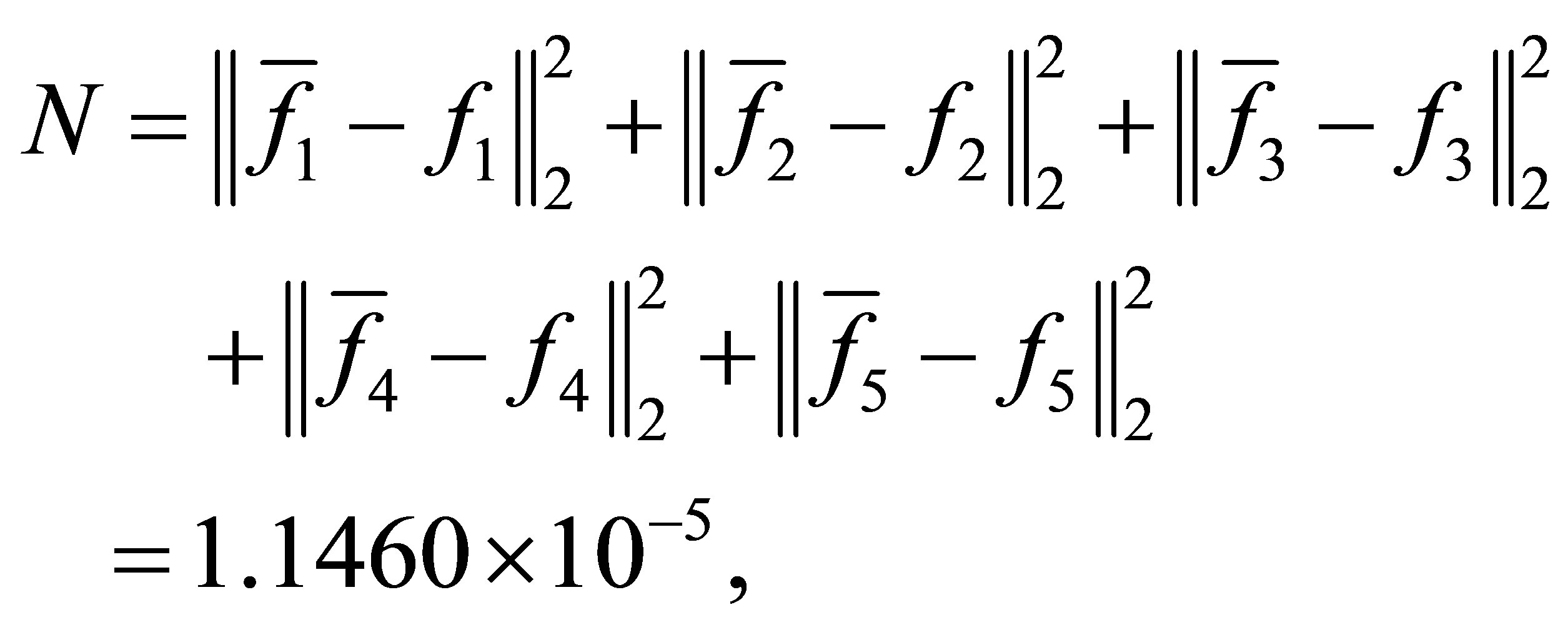
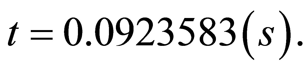
Example 4.3. Let ,
,  and
and


after 11 iterations, we have the polynomials


with a minimum distance
and the CPU time
Example 4.4. Let ,
,  and
and


after 1 iteration, we have the polynomials


with a minimum distance
and the CPU time
Example 4.5. Let ,
,  and
and


after 1 iteration, we have the polynomials


with a minimum distance
and the CPU time
Examples 4.1, 4.2, 4.3, 4.4 and 4.5 show that Algorithm 4.1 is feasible to solve Problem 1.1.
In Table 1, we present the performance of Algorithm 4.1 and compare the accuracy of the new fast algorithm with the algorithms in [9,21]. Denote  be the total degree of polynomials
  and
and  be the total degree of polynomials
 . It (Chu) stands for the number of iterations by the method in [14] whereas it (STLN) denotes the number of iterations by Algorithm 4.1. Denoted by error(Zeng) and error (STLN) are the perturbations
 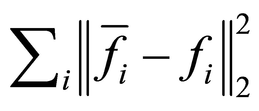 computed by the method in
[21] and Algorithm 4.1, respectively. The last two columns denote the CPU time in seconds costed by AFMP algorithm and our algorithm, respectively.
As shown in the above table, we show that our method based on STLN algorithm converges quickly to the minimal approximate solutions, needing no more than 2 iterations whereas the method in [14] requires more iteration steps. We also note that our algorithm still converges very quickly when the degrees of polynomials become large while the algorithm in [14] needs more iteration steps. Besides, our algorithm needs less CPU time than the AFMP algorithm. So the convergence speed of our method is faster. From the errors, we demonstrate that our method has smaller magnitudes compared with the method in [21]. So our algorithm can generate much more accurate solutions.
5. Conclusion
In this paper, we present that approximation GCD of several polynomials can be solved by a practical and reliable way based on STLN method and transformed to the approximation of Sylvester structure problem. For the matrices related to the minimization problems are all structured matrix with low displacement rank, applying the algorithm to solve these minimization problems would be possible. The complexity of the algorithm is reduced with respect to the degrees of the given polynomials. Although the problem of structured low rank ap-

Table 1. Algorithm performance on benchmarks.
proximation has been studied in many literatures and obtained many accomplishments, there is still much work to be done, for example, low rank approximation of finite dimensional matrix has not been fully resolved.
NOTES