Analytical and Approximate Solutions to the Fee Vibration of Strongly Nonlinear Oscillators ()
1. Introduction
Nonlinear oscillations problem is important in the physical science, mechanical structures and other kind of mathematical sciences. Most of real systems are modeled by nonlinear differential equations which are important issues in mechanical structures, mathematical physics and engineering. Recently, much attention has been focused on the properties to solve nonlinear equations in mechanical systems. In this way, some kind of these methods like Harmonic balance method (HBM) [1], Newton harmonic balance method (NHBM) [2], Frequency-amplitude formulation (FAF) [3-5], Energy balance method (EBM) [6,7], Variational iteration method (VIM) [8,9], Homotopy perturbation method (HPM) [10- 12], Homotopy analysis method (HAM) [13], and MaxMin method (MMA) [14,15] are introduced for nonlinear oscillatory systems.
Our main aim in this paper is to apply a new approach coupled with the iteration method by combining He’s FAF and He’s EBM. We compare the numerical solution with others methods like energy balance method and variational iteration method. We examine accuracy of the approximation methods.
2. Solution Procedure
We consider a generalized nonlinear oscillator in the form:
 (1)
(1)
under the initial conditions:
 (2)
(2)
Based on He’s frequency-amplitude formulation approach [3,4]. The trial function to determine the angular frequency ω is given by
 (3)
(3)
substituting from Equation (3) into Equation (1), one can obtain the following residual as
 (4)
(4)
Introducing a new function,  , defined as [6]
 (5)
(5)
Solving the above equation, the relationship between the amplitude and frequency of the oscillator can be obtained:
3. Applications
In this section, some practical examples for some strongly nonlinear vibration system are illustrated to show the applicability, accuracy and effectiveness of the present method.
3.1. Autonomous Conservative Oscillator
It is known that the free vibrations of an autonomous conservative oscillator with inertia and static type fifthorder non-linearities is expressed by [7,16,17].
 (6)
(6)
The initial conditions for Equation (6) are given by  and
and  where A represents amplitude of the oscillation.
Motion is assumed to start from the position of maximum displacement with zero initial velocity  is an integer which may take values of
 , 0 or −1, and

 and
and  are positive parameters in Table 1.
By using the following trial function to determine the angular frequency :
:
 (7)
(7)
Substituting the above trial functions into Equation (6) results in, the following residual
 (8)
(8)
Using Equation (8) into Equation (5), we can easily obtain
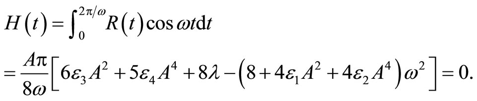 (9)
(9)
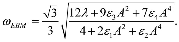
Solving the above equation, an approximate frequency  as a function of amplitude
  as follow:
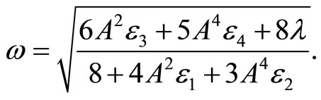 (10)
(10)
Hence, the approximate solution can be readily obtained

Table 1. Values of dimensionless parameters  in Equation (6) for four models [16].
 (11)
(11)
Mehdipour et al. [7] obtained the approximate frequency for Equation (6) by the energy balance method
 (12)
(12)
The values of dimensionless parameters ,
,  ,
,  and
and  associated with each of the four calculation modes are shown in Table 2 [7].
Additionally, the comparison between these methodologies can be found in Table 2 and Figure 1. It has been shown that the results of analytical approximate solution are in good agreement with those obtained from the results of energy balance method [7], and with an accurate numerical solution using fourth-order Runge-Kutta method (R-K) as shown in Table 2 and Figure 1.
3.2. Tapered Beams
Tapered beams is an important model for engineering structures which require a variable stiffness along the length, such as moving arms and turbine blades [18-20]. In dimensionless form, the governing differential equation corresponding to fundamental vibration mode of a tapered beam is given by [20].
 (13)
(13)
Assume that the solution can be expressed as: u(t) = Acosωt.
Similarly, substituting the trial solution into Equation (13), this leads to the following residual
 (14)
(14)
Using Equation (14) into Equation (5) we can easily obtain

Table 2. The comparison between energy balance method [7] and analytical approximate solution for four modes (1 - 4) (λ = 1).


(a) (b) (c) (d)
Figure 1. The comparison between EBM solution (.....), analytical approximate solution (- - -) and numerical solution, solved by the Runge-Kutta method of order 4 (-) for four modes (λ = 1, A = 1).
 (15)
(15)
Solving the above equation, an approximate frequency as a function of amplitude equals:
 (16)
(16)
which is the same as given by Hoseini et al. [20].
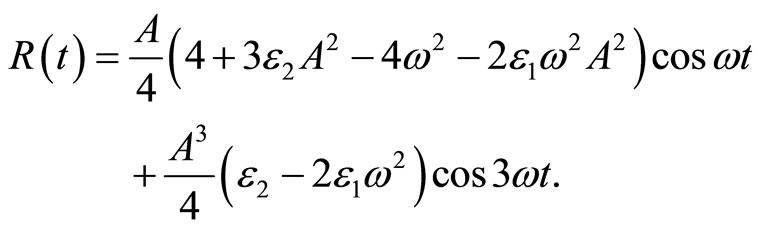
Hence, the approximate solution can be readily obtained
 (17)
(17)
To illustrate the validity of the analytical approximate solution for this example, the results are compared with the variational iteration method [21] and with an accurate numerical solution, using fourth-order Runge-Kutta method (R-K) in Figure 2.

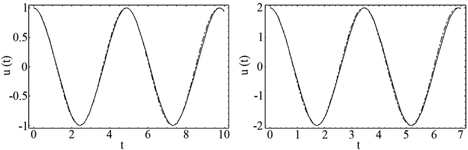
(a) (b) (c) (d)
Figure 2. The comparison between variational iteration method (....), analytical approximate solution (- - -) and numerical solution, solved by the Runge-Kutta method of order 4 (-). (a) Ɛ1 = 0.1, Ɛ2 = 1, A = 1; (b) Ɛ1 = 0.1, Ɛ2 = 1, A = 2; (c) Ɛ1 = 1, Ɛ2 = 2, A = 1; (d) Ɛ1 = 1, Ɛ2 = 1, A = 1.
3.3. Motion of the Particle on Arrange Parabola
The governing equation of motion and initial conditions can be expressed as [5,22-24].
 (18)
(18)
where  and
and  are known positive constants. We choose trial function
 , where
  is assumed to be the frequency of the nonlinear oscillator.
Similar to previous examples we have
 (19)
(19)
Finally, the frequency amplitude relationship can be obtained as:
 (20)
(20)
which is the same as given by Davodi et al. [5]. Hence, the approximate solution can be obtained as
 (21)
(21)
For this following value of parameters the numerical results are compared with EBM [5] and fourth-order Runge-Kutta method (R-K) as shown in Figure 3.
4. Conclusion
The methods to find analytical approximate solutions for nonlinear vibrating equations are not closed, which have important application in physical sciences and engineer-

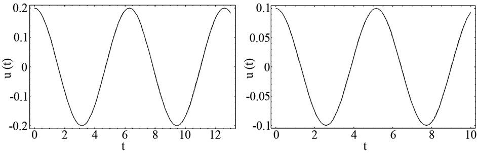
(a) (b) (c) (d)
Figure 3. The comparison between EBM solution (- - -), analytical approximate solution (....) and numerical solution, solved by the Runge-Kutta method of order 4 (-). (a) ∆ = 1, q = 0.2, A = 0.2; (b) ∆ = 1.5, q = 0.6, A = 0.1; (c) ∆ = 1, q = 2, A = 1; (d) ∆ = 1, q = 1, A = 1.
ing. In this way, we illustrated that the present method is very effective and convenient and does not require linearization or small perturbation. The obtained analytical solutions where compared with those calculated by the energy balance method and variational iteration method. The obtained results are valid for the whole solution domain with high accuracy. In comparison to fourth-order Runge-Kutta method, which is powerful numerical solution, the results show that the present method is very convenient for solving nonlinear equations and also can be used for strong nonlinear oscillators.
NOTES