1. Introduction
Sreehari [1] has derived a class of discrete distributions analogous to Burr family by solving a differential equation. The probability mass function (pmf) of the random variable X having the d-th class of the distributions derived by Sreehari (2010) is
 (1)
(1)
with 0 < q < 1.
Nanjundan and Naika [2] have discussed the estimation of the parameter of this distribution.
When this distribution is truncated at 0, the pmf of X turns out to be
 (2)
(2)
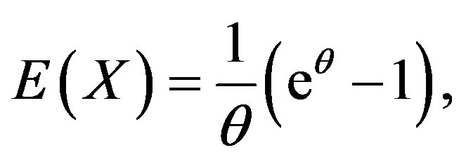
We get

and

It is straightforward to observe that E(X) > Var(X). That is this truncated distribution is under dispersed.
The Fisher information measure is computed in Section 2. The maximum likelihood (ML) estimation of θ is discussed in Section 3 whereas the method of moment estimate of θ is obtained in Section 4. An asymptotic comparison of the maximum likelihood and method of moment estimates is done in Section 5. The results of a simulation study are presented in Section 6.
2. Fisher Information Measure
When X has the pmf specified in (2), we get

Then
and
 .
.
The Fisher information measure corresponding to this pmf is given by

Since the infinite series

is not tractable, it can be numerically evaluated for the required values of θ.
Since Hence,

Therefore,

is convergent and it can be evaluated numerically.
3. Maximum Likelihood Estimation
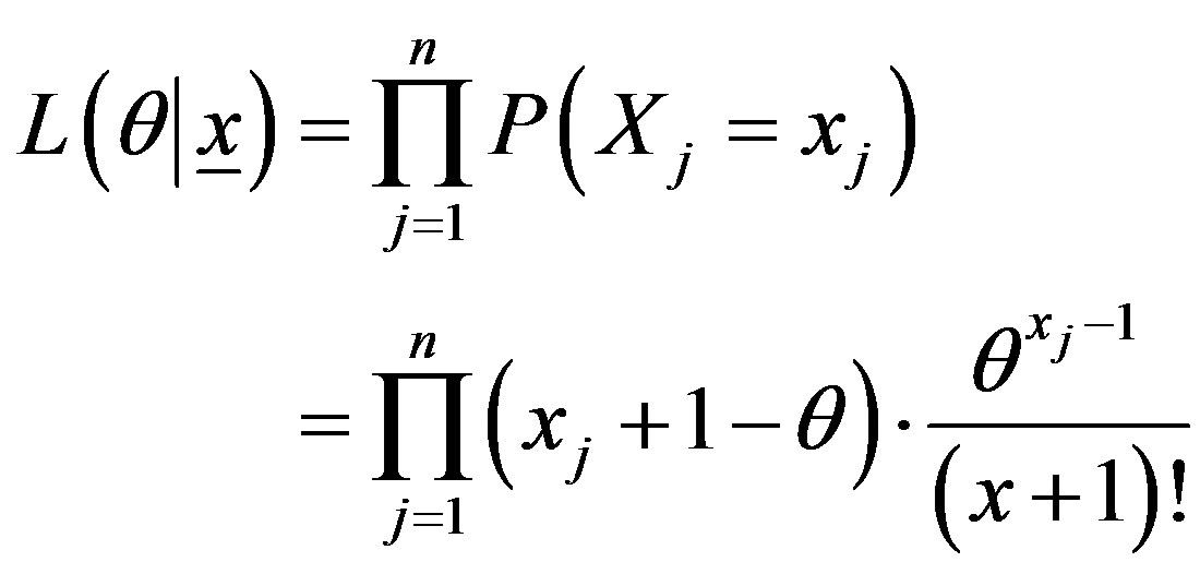
Let  be a random sample on X having the pmf specified in (2). Then the likelihood corresponding to the sample is
The log-likelihood becomes

The maximum likelihood (ML) estimator is given by
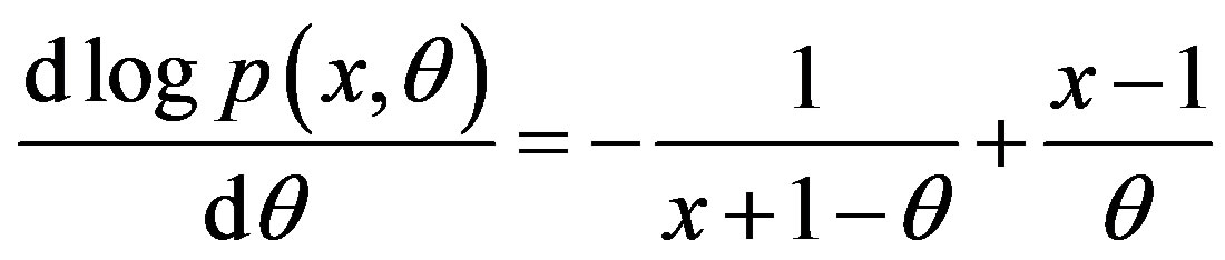
 and hence the ML estimator of θ is the solution of
 . (3)
. (3)
Since (3) does not yield a closed form expression for the ML estimator, it can be evaluated by a numerical procedure like Newton-Raphson method. Let  denote the ML estimator of θ.
The pmf in (2) satisfies the following regularity conditions.
1) The support  of X does not depend on the parameter θ.
2) The parameter space (0, 1) is an open interval.
3) logp(x, θ) is twice differentiable w.r.t. θ.
4)

is twice differentiable w.r.t. θ under the summation sign.
5) There exists a function  such that

and

The conditions 1)-5) are easy to verify. We prove the validity of 5).
Here

since 

where is the true value of the parameter. Since the parameter space is an open interval such a neighborhood exists. Obviously,
Therefore, p(x, θ) satisfies all the regularity conditions of Cramer [3] and it belongs to Cramer family.
Hence

In other words,  is consistent and asymptotically normal (CAN) for θ.
4. Method of Moment Estimation
Let  be a random sample on X having the pmf specified in (1.2) and

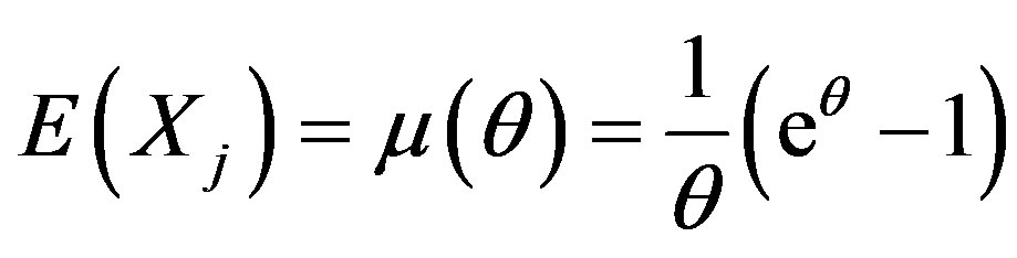
be the first moment of the sample. Since
the method of moment (MM) estimator of θ is given by
 . (4)
. (4)
Evidently the above equation does not admit a closed form expression of the MM estimator of θ and hence for an observed sample, it has to be numerically computed. Let  denote the moment estimator of θ.
Since p(x, θ) does not belong to exponential family, the asymptotic normality of  is not automatic. We establish this property using the delta method.
Note that  are independent and identically distributed (iid) with
and

Note that  is the moment estimate of θ.
By Levy-Lindeberg central limit theorem,

Consider the transformation  Then
Then
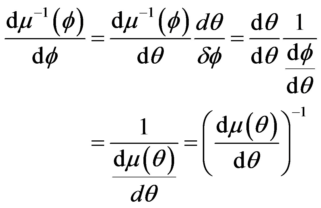
Also
Here


Therefore,
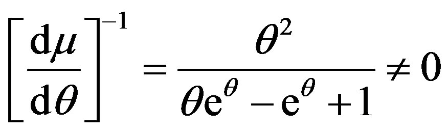
and is continuous.
Hence by the delta method (see Knight [4]),

that is  is also CAN for θ.
5. Asymptotic Relative Efficiency
The asymptotic relative efficiency of the ML estimator over the method of moment estimator is given by

Since the asymptotic variance of  has no closed form expression and is computed numerically, the ARE has also to be numerically evaluated. The table 1 shows the ARE for various values of θ.
The ARE of the ML estimator over the MM estimator is steadily increasing as θ increases. That is the ML estimator uniformly performs better than the MM estimator.
6. Simulation Study
A modest simulation study has been carried out using the R software. One thousand samples, of size 100, 250, and 500 were generated from the truncated distribution specified in (2) for θ = 0.5. Both the ML and the MM estimates were computed solving respectively (3) and (4) using Newton-Raphson method. Sample means were taken to be the initial estimates. Since the asymptotic normality of both estimates has been analytically established, an elaborate simulation study has not been done. However the following histograms give graphical evidence of the asymptotic normality of the estimates. As the sample size increases, the estimates tend to be distributed more normally.
The Figures 1-3 show the histograms of the MLEs and the MMEs based on 1000 samples of sizes 100, 250, and 500 and θ = 0.5.

Table 1. The ARE of the MLE over the MME.

Figure 1. The histograms of the MLEs and the MMEs for sample size 100.

Figure 2. The histograms of the MLEs and the MMEs for sample size 250.

Figure 3. The histograms of the MLEs and the MMEs for sample size 500.
7. Discussions and Summary
The distribution discussed in this paper is structurally similar to the truncated Poisson distribution and under dispersed. Hence this distribution can be used as an alternative to the truncated Poisson when the data exhibit under dispersion.
Both the ML and MM estimators do not have closed form expressions. But they can easily be computed using Newton-Raphson method. Both of the estimators are CAN for the parameter. The ML estimator is asymptotically more efficient than the MM estimator.
8. Acknowledgements
The author is grateful to the referee and Prof. B. Chandrasekar whose suggestions improved the presentation of the results.