Numerical Solution for a Similar Flow between Two Disks in the Presence of a Magnetic Field ()
1. Introduction
The quest for similar solutions is particularly important with respect to the mathematical character of the solution. In cases where similar solutions exist, it is possible, to reduce the system of partial differential equations to one involving ordinary differential equations, which evidently constitute, a considerable mathematical simplifycation of the problem. Wang [1] studied a viscous fluid between two parallel plates, which are being squeezed or separated with normal velocity proportional to  and found similarity solutions of the unsteady Navier-Stocks equations. Ishizawa [2] derived a similarity solution to the case of the unsteady laminar flow between two parallel disks. Tichy and Bourgin [3] found that a similarity solution does exist for the steady flow in a narrow channel of a gap width varying as
 , where
  and
and  are constants. Bhupendra et al. [4] considered the problem of forced flow of an electrically conducting viscous incompressible fluid due to an infinite rotating disk under the influence of uniform magnetic field, applied normal to the flow. Pavlov [5] found an exact similarity solution of MHD boundary layer equations for the steady two dimensional flow of an electrically conducting incompressible fluid due to rotation of a plane elastic surface in the presence of a uniform transverse magnetic field. Guria et al. [6] obtained exact solution of hyderomagnetic flow between two porous disks rotating with same angular velocity about two non coincident axes in the presence of a uniform transverse magnetic field. Attia [7] studied the problem of steady flow and heat transfer of a conducting fluid due to the rotation of an infinite, non conducting porous disk in the presence of an external magnetic field. Sajid et al. [8] examined the MHD rotating flow of a viscous fluid over a shrinking sheet. Asir et al. [9] gave a new hybrid analytical algorithm to study the effects of uniform suction of a laminar, steady, incompressible magnetohyderodynamic electrically conducting fluid over a rotating disk. The purpose of present study is to obtain numerical solution for similar flows of a Newtonian fluid between two disks in the presence of a magnetic field. Usha and Vasudevan [10] studied a similar flow between two rotating disks in the presence of a magnetic field and obtained rather expensive solution of the problem to observe the effect of flow parameters on the velocity fluid.
2. Mathematical Analysis
It has been assumed the flow is axisymmetric, incomepressible and non-steady. The flow is between two parallel infinite disks, which are separated a distance  apart, where
  denotes time. A magnetic field of strength
  is applied perpendicular to the two disks. The upper disk is moving with velocity
  towards the lower fixed disk. Cylindrical polar coordinates
  are used. The lower disk is at
  and the upper one is at
  where
where .
.
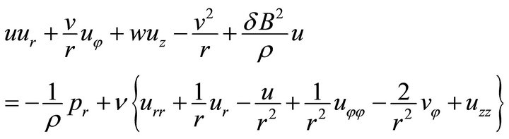
The equations of motion in component form become as follows:
 (1)
(1)
 (2)
(2)
 (3)
(3)
 (4)
(4)
where the subscripts denote the partial differentiation with respect to space coordinates  is the density,
  the pressure and
  the coefficient of kinematics viscosity.
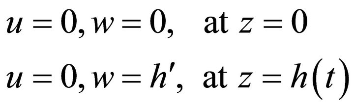
The boundary conditions are:
 (5)
(5)
The following similarity transformations are used:


where
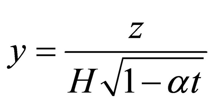
is the dimensionless variable. The equation of continuity is identically satisfied. Equations (2) and (3) take the forms below respectively.
 (6)
(6)
 (7)
(7)
where ,
,  , here
  denotes viscosity and
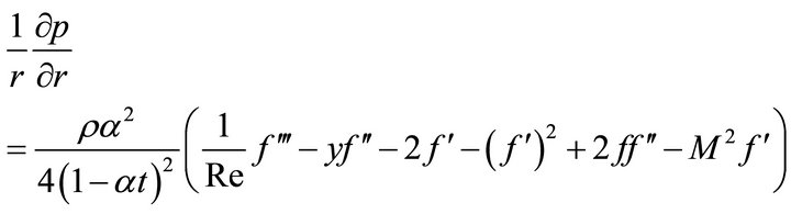
  denotes fluid electrical conductivity. Whence the differentiation of Equation (6) with respect
  and that of Equation (7) with respect to r yield:
 (8)
(8)
Equation (8) is integrated to get:
 (9)
(9)
where  is constant of integration.
The boundary conditions in dimensionless form become;
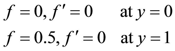 (10)
(10)
3. Finite-Difference Equations
In order to solve Equation (9) numerically, we let
 , (11)
and we obtain
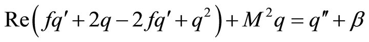 (12)
(12)
The boundary conditions (10) become as:
 (13)
(13)
The derivatives involved in Equation (12) are approximated by central difference approximation at a typical point  of interval [0,1], we get.
 (14)
(14)
where  denotes a grid size and Equation (11) is integrated numerically. Also the symbols used denote
  and
and 
4. Computational Procedure
Finite difference Equation (14) and the first order ordinary differential Equation (11) are solved simultaneously by using SOR method Smith [11, p.262] and Simpson’s (1/3) rule Gerald [12, p.293] with the formula given in Milne [13, p.48] respectively subject to the appropriate boundary conditions.
The order of the sequence of iterations is as follows:
1) The Equation (14) for the solution of  is solved subject to the boundary conditions (13).
2) For the solution of  we use the computed values of
  from above step in to Equation (11) and integrate by Simpson’s (1/3) rule.
3) The optimum value of the relaxation parameter  is estimated to accelerate the convergence of the SOR method.
4) The SOR procedure is terminated when the following criterion is satisfied for q:
 where
where  denotes the number of iterations and
  stands for q.
The above steps 1 to 4 are repeated for higher grid levels  and
and . The SOR procedure gives the solution of
  of order of accuracy
  due to second order finite differences used to approximate the derivatives while Simpson’s (1/3) rule gives the order of accuracy
  in the solution of
 . Higher order accuracy in the solution of
  on the basis of above solutions is achieved by using Richardson’s Extrapolation Burden [14, p.168]. The solution of order of accuracy
  in the following tables for computation of
  is the most accurate and accepted solution.
5. Results and Discussion
The numerical solutions examine the way in which the flow pattern changes with the squeeze Reynolds number Re and Hartmann number M. Hamza [15] investigated this problem for the range , 0.0 < M ≤ 30.0. We extended the previous work and analyzed the problem for the parameters involved in the range
  and
and .
.
Table 1 shows the values of different parameters used in the numerical procedure. The numerical results for  have been computed for different values of flow parameters namely Re and
 . The accuracy of numerical results is checked by comparing the results on three different grid sizes namely h = 0.025, 0.012 and 0.006. The comparison of
  is shown in the Tables 2- 4 using Richardson extrapolation method. Graphically, the results have been demonstrated in Figures 1-6. It is found that for fixed Re, there is a slight increase in the

Table 1. Optimum value of relaxation parameter used in SOR method.
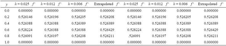
Table 2. M = 40.0, Re = 0.01, M = 50.0, Re = 0.01.
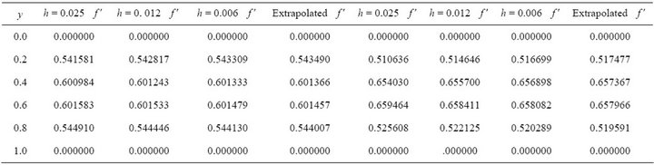
Table 3. M = 10.0, Re = 10.0, M = 0.0, Re = 15.0.
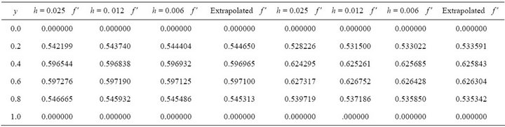
Table 4. M = 10.0, Re = 15.0, M = 5.0, Re = 20.0.

Figure 1. Graph of  for different values of M when Re = 0.01.

Figure 2. Graph of  for different values of M when Re = 1.0.
value of  near the disks and a slight decrease in the region of the mid plane with increase in
 . This in-
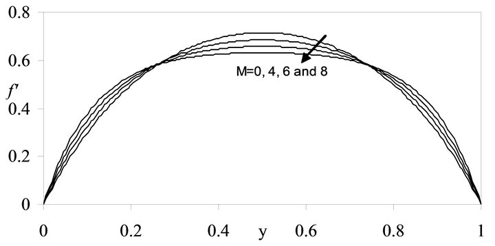
Figure 3. Graph of  for different values of M when Re = 5.0.

Figure 4. Graph of  for different values of M when Re = 10.0.
crease and decrease become more prominent with more increase in , also the radial velocity profiles become more flat in the interior region for all values of Re. On
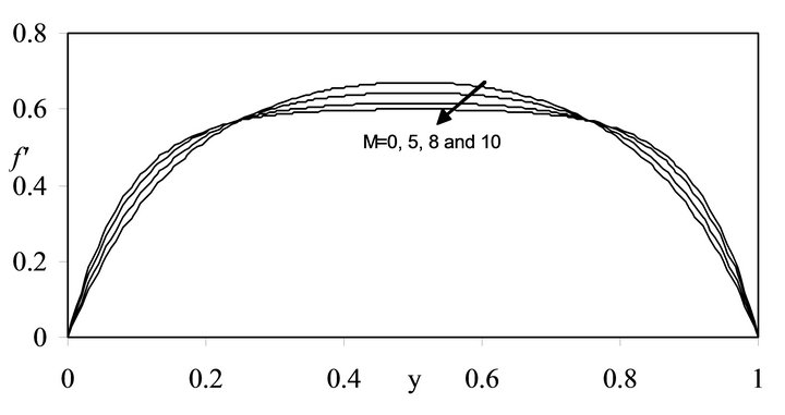
Figure 5. Graph of  for different values of M when Re = 15.0.

Figure 6. Graph of  for different values of M when Re = 20.0.
the other hand, for fixed values of , the magnitude of radial flow decreases with increase in Re. The value of
  is determined by hit and trial to satisfy the approximate zero-order perturbation results given in [15] as
 .
.