Bifurcation Analysis of a Stage-Structured Prey-Predator System with Discrete and Continuous Delays ()
1. Introduction
In the natural world, there are many species whose individual members have a life history that takes them through two stages: immature and mature. In 1990, Aiello and Freedman [1] introduced single-species stagestructured model with time delay, and the stability of the system was studied. In 1997, Wang and Chen [2] introduced single-species stage-structured model without time delay and found that an orbitally asymptotically stable periodic orbit existence. In these papers [3], the authors assume that the life history of each population is divided into distinctive stages: the immature and mature members of the population, where only the mature member can reproduce themselves. However, in the nature many species go through three life stages: immature, mature and old. For example, many female animals lose reproductive ability when they are old.
A single species with three life history stage and cannibalism model have considered by S. J. Gao [4], and shown that the stability of the positive equilibrium can change a finite number of times at most as time delay is increased when the model under some parameters values. Recently, a nonautonomous three-stage-structured predator-prey system with time delay have studied by S. J. Yang and B. Shi [5], by using the continuation theorem of coincidence degree theory, the existence of a positive periodic solution is obtained. And the local Hopf bifurcation and global periodic solutions for a delayed threestage-structured predator-prey considered by Li et al. [6, 7].
2. Formulation of the Model
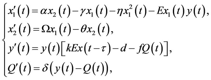
In this paper, we consider following three-stage-structured prey-predator model with discrete and continuous time delays
 (2.1)
(2.1)
where
 are the densities of immature preys, mature preys and old preys population at time
  is the density of predator population at time t, respectively. All of the parameters are positive,
  is the birth rate of mature prey population, and
  are the death rate of immature, mature and old prey population, respectively.
  and
and  are the maturity rate and ageing rate of the prey population, respectively.
  and
and  are the density dependent coefficients of immature prey population and predator population, respectively.
  is the rate of conversing prey into predator and
  is the predation coefficient.
  and
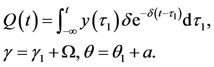
and  are the gestation delay and density dependent for predator population, respectively.
Note that in (2.1),  is linear dependent on
 . That is, the asymptotic behavior of
  is dependent on
 . Therefore, we just need to study following subsystem
 (2.2)
(2.2)
where
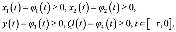
The initial conditions for (2.2) are
3. Local Stability Analysis and Hopf Bifurcation
3.1. Local Stability Analysis
Obviously, system (2.2) has two boundary equilibrium ,
,  (if condition
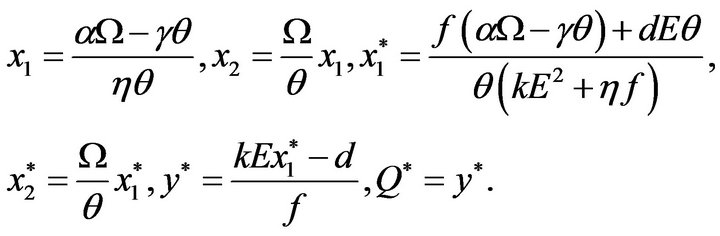
 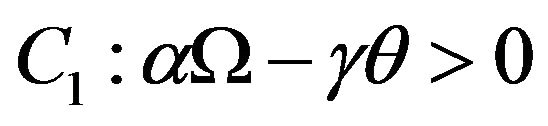 holds), and an unique positive equilibrium
  (if condition
  holds), where
Let ,
,  be any arbitrary equilibrium. The linearized equations are
 (3.1)
(3.1)
where
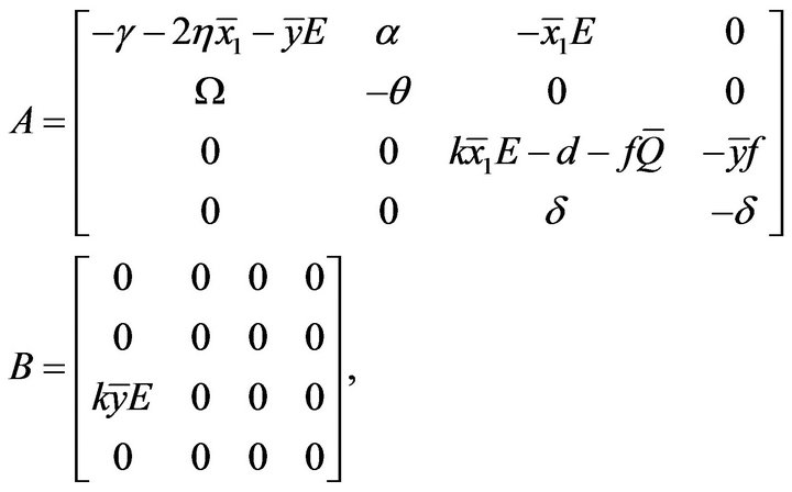
and the characteristic equation about  is given by
 (3.2)
(3.2)
Theorem 1. 1)  is local stable if
 , local unstable if
  and
and  exist.
2)  is local stable if
 , local unstable if
  and
and  exist.
Proof. 1) From (3.2), the characteristic equation about  is given by
 (3.3)
(3.3)
Then,  , and
, and  are the two other roots of
By Routh-Hurwitz criterion,  is local stable if
 , local unstable if
  and
and  exist.
2) From (3.2), the characteristic equation about  is given by
 (3.4)
(3.4)
Then,  are the two roots of
with negative real parts. , by Routh-Hurwitz criterion,
  is local stable if
 , local unstable if
  and
and  exist.
3.2. Existence of Local Hopf Bifurcation
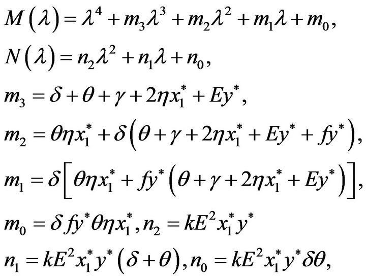
The characteristic equation about the positive equilibrium  is given by
 (3.5)
(3.5)
where
When , (3.5) becomes to
 (3.6)
(3.6)
and  Note that
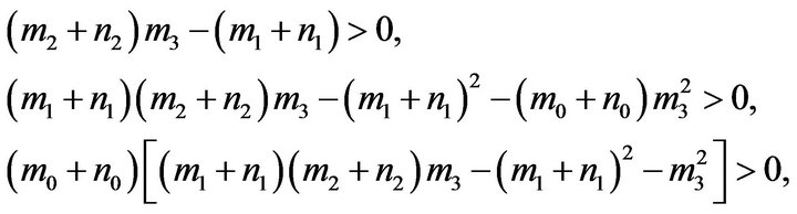
if condition  holds. By Routh-Hurwits criterion, all roots of (3.6) have negative real parts. Then, the equilibrium
  is local stable.
Suppose ,
,  is a root of (3.5) and separating the real and imaginary parts, one can get that
 (3.7)
(3.7)
From (3.7), we have
 (3.8)
(3.8)
namely
 (3.9)
(3.9)
where
If condition  hold, then
 , (3.9) have at least one positive root. Without loss of generality, we assume (3.9) have four distinct positive roots
 , then (3.5) have four pair of imaginary roots
 . From (3.7), we have
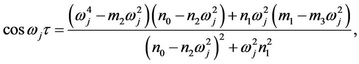
Thus, the corresponding to
  are given by
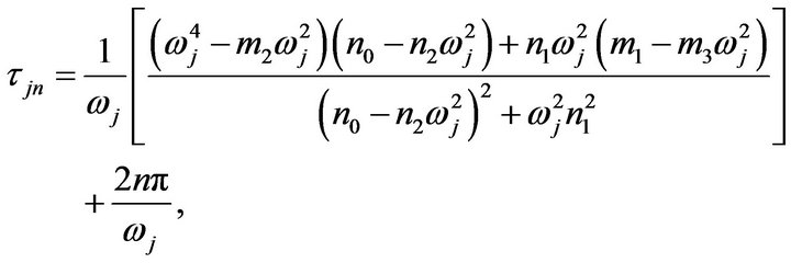 (3.10)
And the direction of  pass through the imaginary axis [8] when
  is given by

Then , since
  four distinct positive roots of (3.9). Let
 (3.11)
According to the Hopf bifurcation theorem for functional differential equations [9], (2.2) can undergoes a Hopf bifurcation at the positive equilibrium  when
when . Furthermore, if condition
 ,
,  holds, then (3.9) have unique positive root
 , and the
  corresponding to
  are given by
 (3.12)
and , according to the Hopf bifurcation theorem for functional differential equations [9], (2.2) can undergoes a Hopf bifurcation at the positive equilibrium
  when
when . Based on above analysis, we have the following result.
Theorem 2. 1) If condition  holds, then there exists a
 , when
  the positive equilibrium
  of (1.2) is asymptotically stable and unstable when
 , where
  is defined by (2.11).
2) If condition  holds, then there exists a
 , when
  the positive equilibrium
  of (2.2) is asymptotically stable and unstable when
 , (2.2) can undergoes a Hopf bifurcation at the positive equilibrium
  when
when , where
  is defined by (3.12).
Remark 1. It must be pointed out that Theorem 2 can not determine the stability and the direction of bifurcating periodic solutions, that is, the periodic solutions may exists either for  or for
 , near
 . To determine the stability, direction and other properties of bifurcating periodic solutions, the normal form theory and center manifold argument should be considered [10].
4. Numerical Simulation
We consider following stage-structured delay system
 (4.1)
(4.1)
where
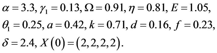
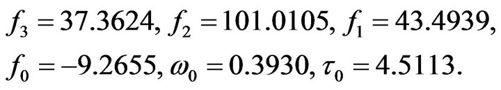
System (4.1) has an unique positive equilibrium point . We solve model (4.1) using function dde23 in MATLAB, and compute that
According to Theorem 2, the positive equilibrium point E2 is asymptotically stable when  (see Figure 1). When
 , the positive equilibrium point E2 is unstable and the Hopf bifurcation occurring around the positive equilibrium E2 are shown (see Figure 2). The bifurcating periodic solution (limit cycle) of (4.1) are stable when
  (see Figure 3), the amplitudes of period oscillatory are increasing as time delays increased. But, too large time delay would make the population to be die out, because the population very close to zero as time delay increase to some critical value.
5. Conclusion
In this paper, we considered a three-stage-structured prey-predator system with discrete and continuous time delays and analyzed the stability of the boundary and positive equilibrium, obtained the conditions of the positive equilibrium occurring Hopf bifurcation by analyzing the characteristic equation about it. Numerical examples by time-series plot have shown that the system considered local asymptotically stable when  and stable Hopf bifurcation periodic solutions when
  and
and  near
near . That is to say, time delay can make the positive equilibrium lose stability. It is shown that populations can be coexistence with periodic fluctuating under some conditions and such fluctuation is caused by the time delay. The bifurcating periodic solution (limit cycle) is stable when
  from 5 to 40 and the amplitudes of period oscillatory are increasing as time delays increased. But, too large time delay would make the population to
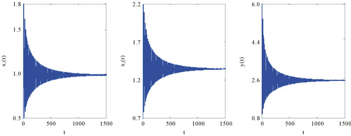
Figure 1. The time-series plot show that positive equilibrium point E2 of (4.1) are asymptotically stable for τ = 4.4 < τ0.
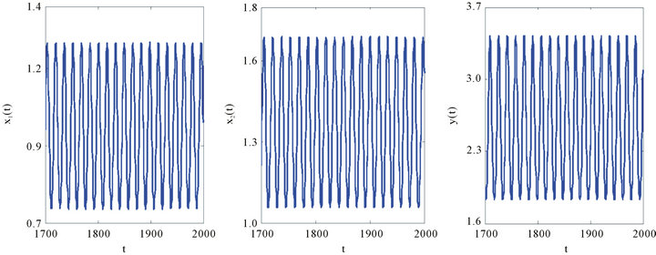
Figure 2. The time-series plot show that (4.1) undergoes Hopf bifurcation for τ = 4.6 > τ0.
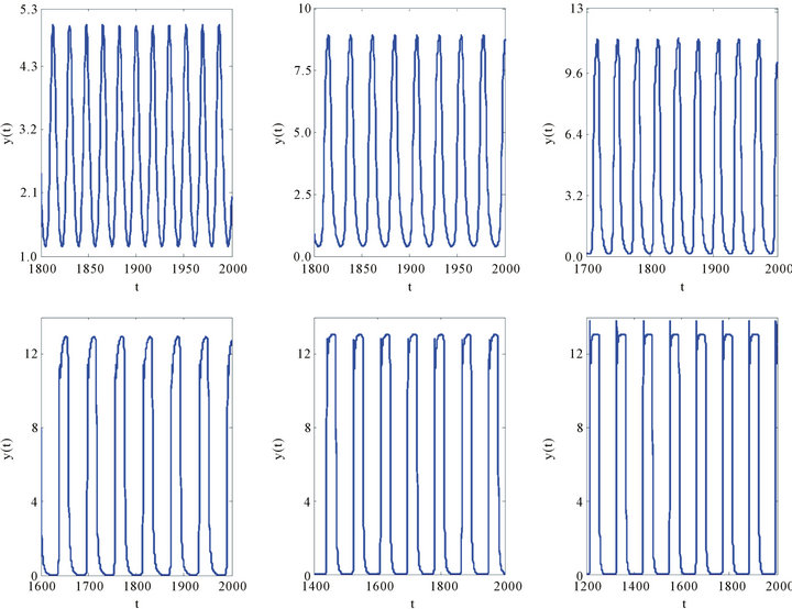
Figure 3. The Hopf bifurcating periodic solution (limit cycles) of (4.1) when τ = 5, 7, 10, 20, 30, 40.
be extinct, because the population arbitrary close to zero as time delay increase to some critical value. These are very interesting in mathematics and biology.
6. Acknowledgements
This work was supported by the Natural Science Foundation of Guizhou Province (No. [2011] 2116).