A Conventional Approach for the Solution of the Fifth Order Boundary Value Problems Using Sixth Degree Spline Functions ()
1. Introduction
In the recent past, several authors have considered the application of cubic spline functions for the solution of two point boundary value problems. Bickley [1] has considered the use of cubic spline for solving second order two point boundary value problems. The essential feature of his analysis is that it leads to the solution of a set of linear equations whose matrix coefficients are of upper Heisenberg form. Bickley uses a special notation other than the conventional one for the representation of the cubic spline, for a detailed discussion one may refer to E. A. Boquez and J. D. A. Walker [2], M. M. Chawla [3], and P. S. Ramachandra Rao [4-7]. We used Bickley’s method for the construction of a sixth degree spline and apply it to the linear fifth order differential equation with two different problems with different boundary conditions. The work has been illustrated through examples with h = 0.5 and h = 0.25.
2. Cubic Spline-Bickley’s Method
Suppose the interval  is divided in to n subintervals with knots
  starting at
 , the function
  in the interval
 is represented by a cubic spline in the form

(1)
Proceeding in to the next interval , we add a term
 ; proceeding in to the next interval
 , we add another term
  and so until we reach
 . Thus the function
  is represented in the form for
(1.1)
(1.2)

(1.3)
2.1. The Two-Point Second Order Boundary Value Problem
First, we consider the linear differential equation

(1.4)
With the boundary conditions
(1.5)
The number of coefficients in (1.1) is (n + 3). The satisfaction of the differential equation by the spline function at the (n + 1) nodes gives (n + 1) equations in the (n + 3) unknowns. Also the end conditions (1.5) give us two more equations in the unknowns. Thus we get (n + 3) equations in (n + 3) unknowns . after determining these unknowns we substitute them in (1.1) and thus we get the cubic spline approximation of
 . Putting
 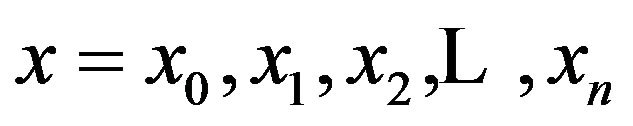 in the spline function thus determined, we get the solution at the nodes. The system of equations to be satisfied by the coefficients
  are derived below.
Substituting (1.1), (1.2), (1.3) in (1.4), at  we get

(1.6)
where  and so on. Applying boundary conditions in (1.5), we get
 (1.7)
(1.7)
If these equations are taken in the order (1.7), (1.6) with , the matrix of the coefficients of the unknowns
  is of the Heisenberg form, namely an upper triangle with a single lower sub-diagonal. The forward elimination is then simple, with only one multiplier at each step and the back substitution is correspondingly easy.
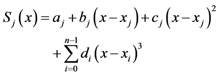
2.2. Construction of the Sixth Degree Spline
Suppose the interval  is divided in to “n” subintervals with knots
 . Starting at x0, the function
  in the interval
  is represented by a sixth degree spline

Proceeding in to the next interval , we add a term
 , Proceeding in to the next interval
  we add another term
  and so until we reach
 . Thus the function
  is represented in the form

(1.8)
It can be seen that  and its first five derivatives are continuous across nodes.
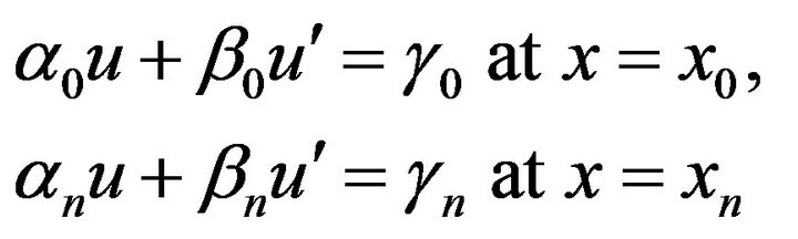
3. Fifth Order Boundary Value Problem
We consider the linear fifth order differential equation

(1.9)
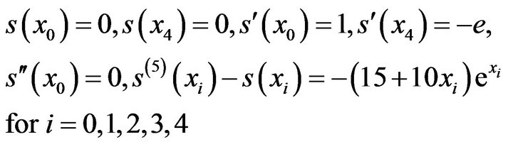
With the boundary conditions

(1.10)
We get (n + 6) equations in (n + 6) unknowns ,
, . After determining these unknowns we substitute them in (1.8) and thus we get the sixth degree spline approximation of
 . Putting
  in the spline function thus determined, we get the solution at the nodes. The system of equations to be satisfied by the coefficients
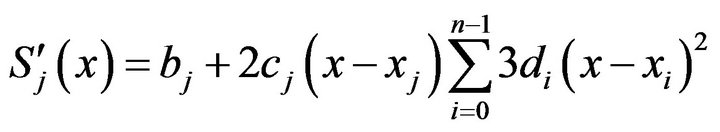
 are derived below. From (1.8) we get

(1.11)
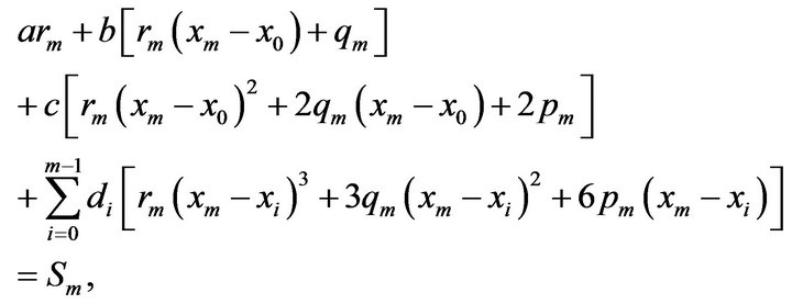
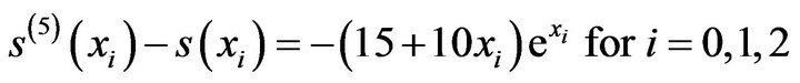
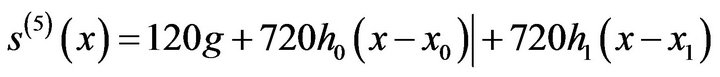
using (1.8) & (1.11) in the differential Equation (1.9) at the nodes  takes of the form
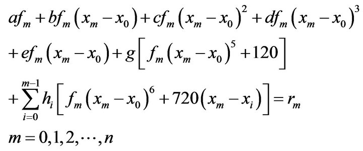
(1.12)
To these equations we add those obtained from the boundary conditions (1.10), we get
(1.13)

(1.14)

(1.15)

(1.16)

(1.17)
If these equations are taken in the order (1.14), (1.16), (1.12) with , (1.17), (1.15) & (1.13) the matrix of the coefficients of the unknowns,
  ,
,  is an upper triangular matrix with two lower sub diagonals. The forward elimination is then simple with only two multipliers at each step, and the back substitution is correspondingly easy.
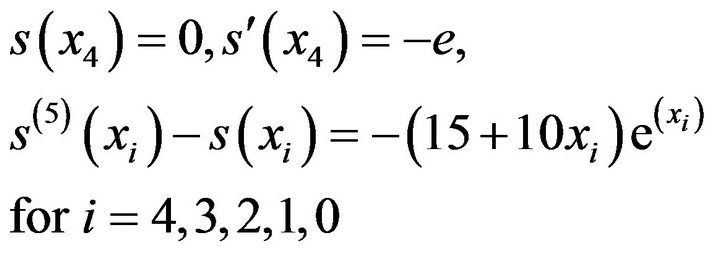
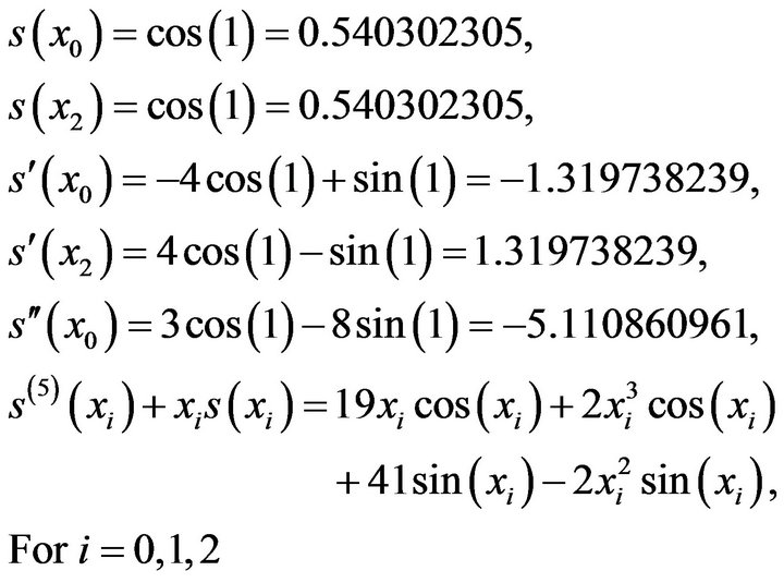
3.1. Example 1
Consider the following fifth order linear boundary value problem

(1.18)
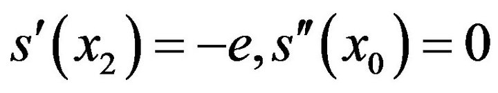
With the boundary conditions

(2)
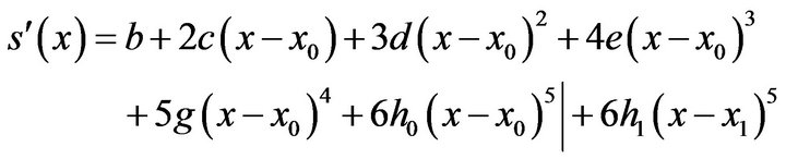
by taking equal subintervals with h = 0.5 and h = 0.25 1) Solution with h = 0.5 The sixth order spline  which approximates
  is given by

(3)
where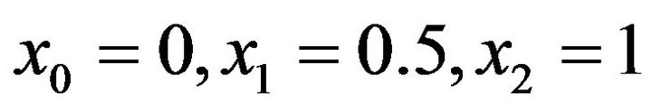 . We have eight unknowns
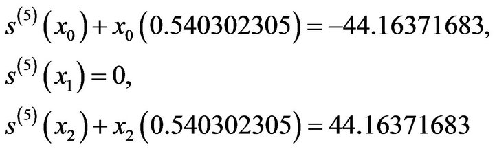
  and eight conditions to be satisfied by these unknowns are
 ,
,
(4)
(5)
Since 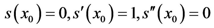 it follows that
  Equation (3) reduces to the form

(6)
also since  and equations of (5) for i = 0 & 2 reduces to
 and
and 
It follows that we have to determine the five unknowns  in Equation (6), subject to the five conditions

(7)
from (6)
(8)
and

(9)
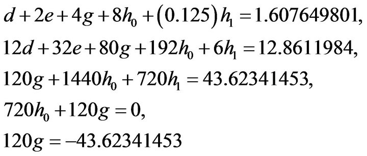
Substituting (6), (8), (9) in (7) we get the system of equations
(10)
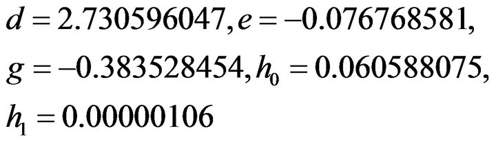
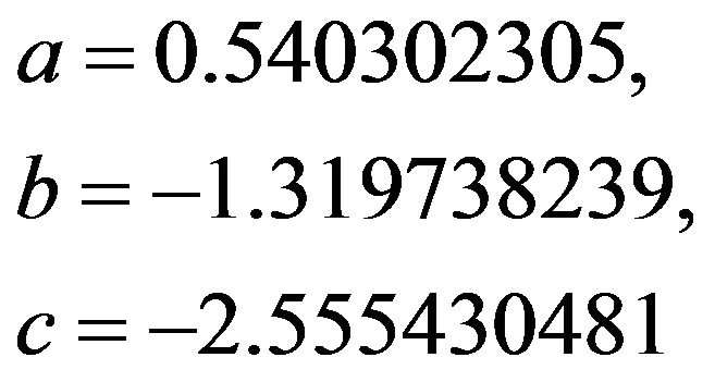
Solving these we get

Substituting these values in (6) we get

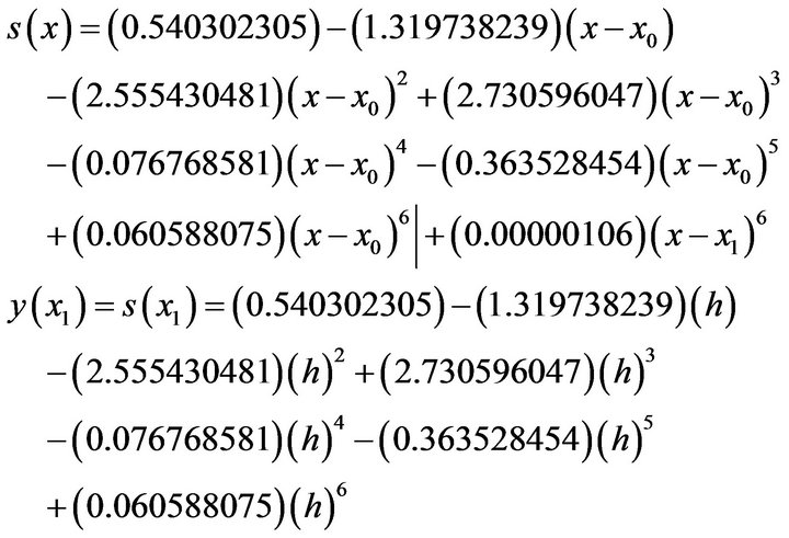
(11)

where h = 0.5 Therefore 
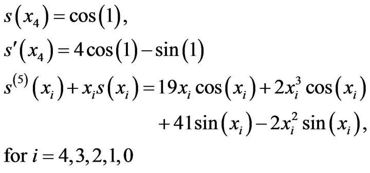
The analytical solution of the differential equation (1.18) subject to the conditions is given by

(11.1)
The exact value of 
It follows that the Absolute error of the numerical value of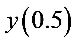 , computed from the spline approximation is 0.00083433 which is very small.
2) Solution with h = 0.25
The interval [0,1] is divided in to 4 equal subintervals we denote the knots by  where
where ,
, .
.
The sixth order spline  which approximate
  is given by

(12)
There are 10 unknowns in  which are to be determined from 10 conditions
(13)
In view of the conditions 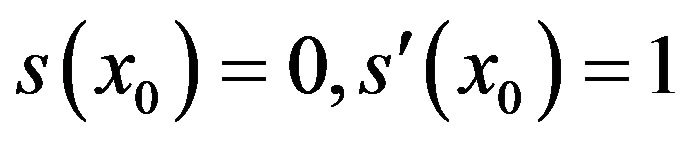 and
and  it follows that
  hence The spline
  reduces to the form

(14)
From (14)

(15)

(16)
Substituting (14), (15), (16) in (13) taken in the order,
we get the following system of equations
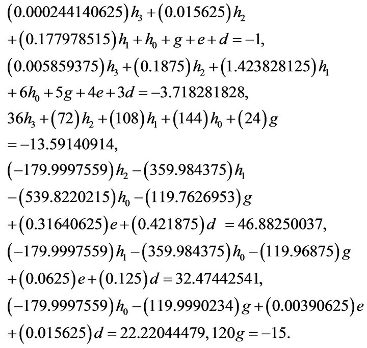
(17)
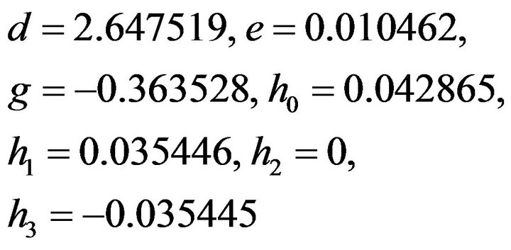
From the above system of equations, we notice that the coefficient matrix is an upper triangular matrix with two lower sub diagonals. solving the above equations we get

(18)
However it may be noticed that from the Equation (17)  which when substituted in the remaining equations will give us a 6 × 6 system of equations which may be solved. Substituting (18) in (14) we get the spline Approximation
  of
of . The values of
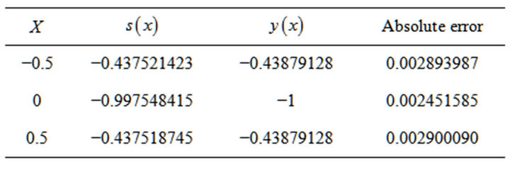
 , and The corresponding absolute errors at
  tabulated in Table 1.
The analytical solution of the differential equation (1.18) with the conditions is given by (11.1) is symmetric about the central value. The same aspect is also satisfied by the numerical approximations as is evident from the above table. We found that the approximate values are remarkably accurate.
3.2. Example 2
Consider the following fifth order linear boundary value problem
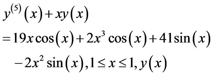
(19)
Subject to

(20)
1) Solution with 
The sixth order spline  which approximates
  is given by (3). The equations to be satisfied by the coefficients of the spline function are
(21)
We observe that

Table 1. Approximate solutions and absolute errors for Example 1 with h = 0.25.

also since

and  the equations of (21) for
  reduces to
It follows that we have to determine the 5 unknowns 
 in Equation (3), subject to the five conditions

(22)
From (3)
(23)
 (24)
(24)
Substituting (3), (23), (24) in (22)
We get the system of equations
(25)
Solving these we get
also we have

Substituting all these values in Equation (3) we get the spline approximation for  which is given by
(26)
where 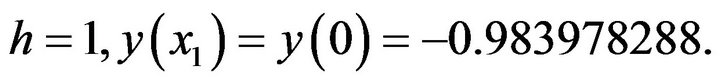
The analytical solution of (19) with the conditions (20) is given by

(27)
The exact value of  it follows that the absolute error in the numerical approximation
  is found to be
 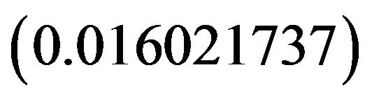 which is very small.
2) Solution with 
The interval  is divided in to 4 equal subintervals we denote the knots by
  where
where 
We assume the spline function  which approximates
  in the form is given by (12)
From (12) we have

(28)
The conditions to be satisfied by  are
are

(29)
for  from (29) we find that
Table 2. Approximate solutions and absolute errors for Example 2 with h = 0.5.
using the remaining conditions of (29) in the order,
that is taking the Equations (12), (16), (28) in (29) & by substituting the values of 
We get the following system of equations

(30)
Solving (29) we get
(31)
Also we have

Substituting these values in (12) we get the approximation .
.
The values of  and the corresponding absolute errors at
  are mentioned in Table 2.
4. Conclusion
Numerical values obtained by the spline approximation have high accuracy. It has been noticed that the numerical solutions obtained are remarkably accurate and have negligible percentage errors even for values of h as large as 0.5, 1.0.
NOTES