The Conservation Laws and Stability of Fluid Waves of Permanent Form ()
1. Introduction
This paper is based on Nekrasov’s integral equation solution obtained in [1,2]. This solution allows us to find the profile and velocity of a gravitational wave, and the calculation of the wave kinetic and potential energy is possible. At fixed depth of fluid the solution of Nekrasov’s integral equation exists on a limited segment of wavelength  The potential and full mechanical energies are monotonically increasing functions on the segment
 . From the law of the change of wave’s kinetic energy presented in [3] as mathematical theorem follows that the kinetic energy vanishes on the boundaries of the segment
  and has the maximum at a point
  Thus we observe symmetry: at the points
  the full mechanical energy consists only of potential energy. The wave of constant shape may be considered as a compound pendulum with a suspension center in the origin of coordinates arranged on unperturbed surface of fluid.Then the wave stability is spotted as a compound pendulum stability.
The plan of the paper is as follows. In Section 2, we describe the method of Nekrasov’s integral equation solution. Here this method has been used for evaluation of the maximum wavelength  boundaries and for estimation of the maximum slope of the wave free surface.
In Section 3, geometrical and energy properties of a wave are explored and the theorem about the change of the wave velocity on the segment  is proved. As a result we have gained the laws of the change of wave’s kinetic and potential energy. Here we have defined the wave’s center of mass as a function of depth-towavelength ratio and have made some suppositions concerning the wave stability considering it as a compound pendulum.
2. Solution of Nekrasov’s Integral Equation
Nekrasov’s integral equation describing steady state waves of unchangeable shape on the surface of a fluid with finite depth  is written as [4]
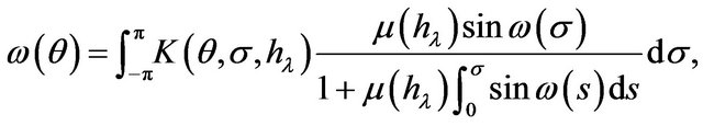 (1.1)
(1.1)
where  - is the polar angle,
  - is the angle that the wave surface makes with the horizontal,
  - is the wavelength,
  - is an arbitrary constant,

From Equation (1.1) follows that required function  represents a trigonometric series
 (1.2)
(1.2)
The evaluation of scalar product
taking account of Equations (1.1) and (1.2) gives a system of  nonlinear integral equations
 (1.3)
(1.3)
where the subscript  denotes that in Equation (1.1) a truncated kernel
  with
with  instead of
  is used. Below the subscript
  of any function will be omitted if
 (1.4)
(1.4)
where  - is a suitable from accuracy point of view small number The system (1.3) containing
  unknowns
  is underdetermined and has a set of solutions including the trivial.
We assume that the first coefficient  is independent of
  and
and  and can be calculated from the linearized on
  system (1.3) at
  Thus
Thus
 satisfy the equation
 (1.5)
(1.5)
This equation has been solved by Kellogg’s method [5] in [1,2]. Let us remark that the Kellogg method was applied to a non-linear integral equation and the discovered solution is not spectral. In accordance with [2], Equation (1.5) has a unique solution (the motionless point) 
Now we fix in (1.3)  and consider
  as the initial approximation of
  After that, the system of
  Equations (1.3) contains n unknowns
  and has a solution that cannot be trivial.It has been shown [1,2] that coefficient
  satisfy system (1.3) at
  if
if
 where
where
 (in [2]
  is designated as
 ).This means that the solution of the system (1.3) at
  exists and is unique if the wavelength
where 
The lower boundary of the segment  on which coefficient
  satisfy system (1.3) at
  can be obtained by solving the system

(1.6)
derived from (1.3) by substitution  If requirements (1.4) are satisfied, then the function
  is defined on the segment
  (see [1]), or on the equivalent segment
 (1.7)
(1.7)
The system (1.6) containing n unknowns
 was solved by successive approximations method at
  limited by computer’s throughput. The results of calculations of
  are given below:

The function  is of low accuracy at the point
  and allows only to write the inequalities
  From these inequalities follows that the maximal wavelength
  is bounded on both sides
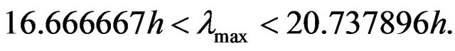
The results of calculations of  for
for  are given below:
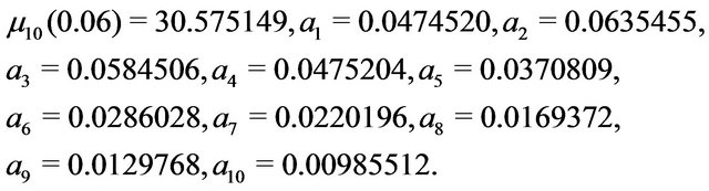
These numerical results assert that  will remain the solution of system (1.3) at
  for any
From the solution of the system (1.6) we obtain the coefficients of the function . This function achieves the maximum
  at the points
 The maximum slope of the free surface in degrees
  exceeds the value
  received in [6]. We suppose that
3. The Conservation Law of Full Mechanical Energy and Stability of a Wave
For evaluation of a wave square and full mechanical energy we need the parametric equations of wave’s surface coordinates
(2.1)
and the function
 (2.2)
(2.2)
Coefficients  are determined as algebraic expressions of
  [2].
[2].
The coordinate origin O is on vertical line through the wave crest at distance h from the bottom,the  axis is directed upward, and the
  axis to the right. In a coordinate system attached to the wave the bottom moves from right to left at velocity [4]
 (2.3)
(2.3)
Using (2.1)-(2.3) at fixed , we obtain the expressions for the properties of the wave: the surface area
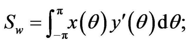 (2.4)
(2.4)
the coordinates of the center of mass
 (2.5)
(2.5)
the kinetic energy
 (2.6)
(2.6)
where constant  denotes the fluid density; the potential energy
 (2.7)
(2.7)
the full mechanical energy
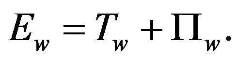 (2.8)
(2.8)
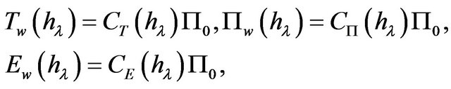
The full mechanical energy of an unperturbed fluid layer with depth h and wavelengths  is considered as
 (2.9)
(2.9)
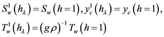
Substituting  for
for  in (2.4)-(2.9), we get

and  where
where
are integrals depending on parameter  Using these relationships we can write the Equations (2.6)-(2.8) in the form
 (2.10)
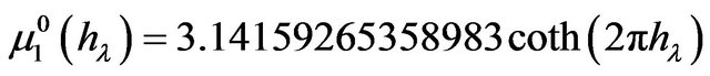
where

The solution of system (1.3) obtained in [2] allow us to calculate the function  on the segment
  On the boundaries of this segment we have

The functions  calculated on the segment
  are shown on Figure 1. The outcomes of these calculations allow to assert that the wave potential energy
  as function of parameter
 monotonically diminishes on the segment
In order to calculate the greatest value of potential energy of a wave we need the  solution of system (1.6) instead of
  (see above).
The law of the wave kinetic energy change is formulated in the form of a mathematical theorem in [3]. This theorem asserts that: 1) for any constant depth of fluid  the wavelength
  2) at the boundaries of the segment
  the wave velocity
 3) there is a value
  at which
 and the wave velocity is maximum, i.e.
Let’s prove the points 1) - 3). 1) From (1.7) follows that  and therefore
2) Suppose the solution  of (1.6) is known and satisfy (1.4). Using this solution we write the integrals
 (2.11)
The first integral is known  the integral
  tends to zero as
  (see [7]). Now it is possible to express the coefficients
  from the system (1.6) in terms of the integrals
  We have
 (2.12)
Taking into account  as
as  from (2.12) follows that series
  is converging independently of convergence or divergence of the series
  Now if we recall (1.7), (2.3), and (2.12), we get

Figure 1. The functions CT(hλ), CII(hλ), CE(hλ) for 0.08 ≤ hλ ≤ 0.4.
Let as remark that the convergence of series  has been proved at a limited
  in [4] and for a
  presented as a converging series in [8].
3) Since the function  vanishes at the boundaries of the interval
  it follows from the Rolles theorem [7] that exists at least a point
 such that
  As the numerator and denominator of right side of Equation (2.3) are strictly increasing functions of
  the point
  is single and
  The values
 have been calculated in [2].
The kinetic energy of the wave vanishes at boundaries of the segment  and reaches the maximum at a point
  (This point is not presented on Figure 1). The full mechanical energy of a wave is a monotonically decreasing function on the segment
 , but vanishes only at the point
  We note also that the profiles of the waves calculated on the segment
  obey the law of mass conservation
The stability of Nekrasov’s waves has been considered in [9]. We proceed from the fact that a liquid maintaining the invariable shape without a vessel, does not suspect that is a fluid.We suppose that a steady state wave can be presented as a compound pendulum with a suspension center in the origin of coordinates. This wave is stable if
 and unstable if
  The function
 is presented on Figure 2. This function has the greatest value
 , is equal to zero
 has the minimum
 and monotonically increases on the interval
  reaching the value
  only at the point
  If we continue to con-
Figure 2. The dependence ych−1(hλ) for 0.08 ≤ hλ ≤ 0.4.
sider the wave behaving as a compound pendulum then it is stable at  and unstable when

In particular let’s consider a wave of length λ = 1000 m on the surface of a fluid with depth  and density
  The solution of system (1.3) at the point
  (see [2]) and the coefficients b1, b2, …, b7 are given below: μ7(0.1) = 7.449619; a1 = 0.047452; a2 = 0.0195554; a3 = 0.00606262; a4 = 0.00183319; a5 = 0.000565461; a6 = 0.000178475; a7 = 0.0000568810; b1 = 0.047452; b2 = 0.0206812; b3 = 0.00700837; b4 = 0.00233431; b5 = 0.000787255; b6 = 0.000268797; b7 = 0.0000921207. Using these outcomes in Formulas (2.1)-(2.10) we get the parameters of the wave: the crest coordinate
  the trough coordinate
  the amplitude
  the coordinates of mass center
  the kinetic energy
  the potential energy
  the velocity
  This wave similar to a tsunami is stable as
For  and
and  (The solution of the system (1.3) and coefficients
  for
for  are given in [2]) the wave parameters will be:


 This wave is unstable as
In summary it is necessary to note that in the accessible publications we have not discovered materials for comparison, except [6].
4. Conclusion
Solving the Nekrasov’s integral equation we avoided the “Liapunov-Schmidt” method and other methods of searching the solution in the neighbourhood of eigenvalues of Nekrasov’s linearized equation. We sought the solution of this equation in the neighbourhood of the motionless point of the nonlinear integral Equation (1.5). This is the point 
 .
.