1. Introduction
In the past, the epidemiology is restricted to the study of morbid phenomena resulting in an increase in sudden sharp and localized in space, the number of cases and time. It focuses primarily on infectious diseases. Epidemiology is a set of methods research by conducting investigations and a decision tool. Infectious diseases are one area where the theoretical were more developed in epidemiology. The mathematical theory of epidemics provides a framework for reconstruction history of past pandemics, contributing to a better understanding transmission mechanisms, a warning earlier vis-à-vis emergent phenomena, and now the prediction of epidemic spread in time and space. Generally, a model contains a disease-free equilibrium and one or multiple equilibria are endemic. The stability of a disease-free status equilibrium and the existence of other nontrivial equilibria can be determined by the ratio called the basic reproductive number, which quantifies the number of secondary infections arise from a simply put infected in a population of sensitive. When the basic reproduction number is less than unity, disease-free equilibrium is locally asymptotically stable, and therefore the disease off after a certain period of time. Similarly, when endemic equilibrium is global attractor, epidemiologically, it means that the disease will prevail and persist in a population and overall stability of these models is relatively low, especially models with delays.
In this paper, we discuss the equilibrium and stability of the model SIQR epidemic with constant infectious period which is made of a delay time. A particular assumption is made that the time which individuals remain infectious can be described by an exponential distribution. This distribution corresponds to the assumption that the chances of recovery in a given time interval are independent of time since infection. To solve the system is the autile decomposition method and for this we use the references of [1-14]. In order to describe the effects of disease immunity temporal delays are often incorporated in such models [15-19].
2. Model Equations
The system is described by equations which are defined as follows:
 (1)
(1)
D’où denotes the population size at time
 ;
; and
and  denote the sizes of the population susceptible to disease, and infectious members, quarantine members and those who were removed from the possibility of infection through temporary immunity, respectively. It is assumed that all new borns are susceptible.
The positive constants  and
and  represent the death rates of susceptible, infectious and those who are being quarantiane and recovered, respectively. Biologically, it is natural to assume that
 . The positive constants
  and
and  represent the birth rate (from insidence) of the population and the recovery rate of infection, respectively. The positive constant
  is the average number of contacts per infective. The positive constants
  are the numbers of transfers or conversions of infected people quarantined and quarantined at recovered. The term
  indicates that an individual has survived to natural death in a pool recovery before becoming susceptible again, where
  is the length of immunity period.
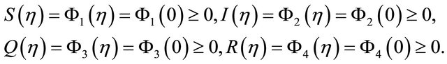
The initial condition of (1) is given as:
 (2)
(2)
where  such that
We have  denote the Banach space
  of continuous functions mapping the interval
  into
into . By a biological meaning, we further assume that
  for
for 
Since  does not appear explicitly in the first three equations of (1), instead of (1) we consider the system:
 (3)
(3)
With the initial condition
 (4)
(4)
where,  we obtain
  and
and
 .
.
The region 
is positively invariant set of (3).
3. The Disease Free Equilibrium and Its Stability
An equilibrium point of system (3) satisfies:
 (5)
(5)
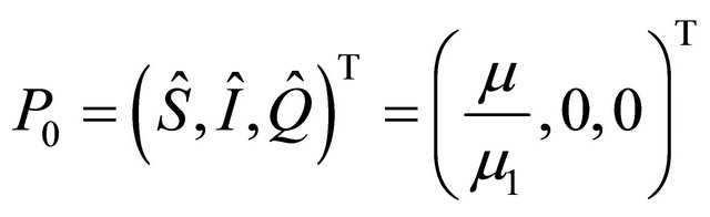
We calculate the points of equilibria in the absence and presence of infection.
In the absence of infection , substituting in the system we obtain the first equilibrium point:
We calculate the Jacobian matrix according to the system (3) with .
.
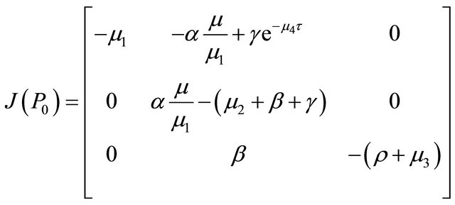
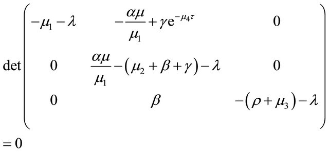
The epidemic is locally asymptotically stable if and only if all eigenvalues of the Jacobian matrix J have negative real part. The eigenvalues can be determined by solving the characteristic equation.
 (6)
(6)
So the three eigenvalues are:
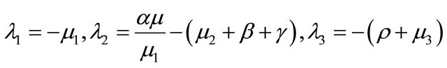
In order for  and
and  to be negative, it is required that
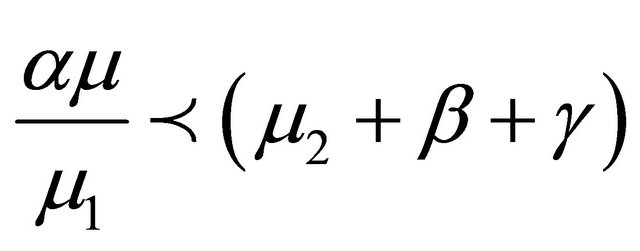 (7)
(7)
Then we define the basic reproduction number of the infection  as follows
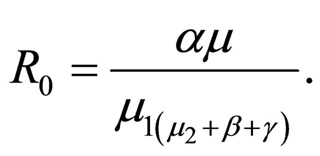 (8)
(8)
3.1. Stability of Equilibrium Point 
The basic reproduction number  is defined as the total number of infected population in the resulting subinfected population where almost all of the uninfected.
Theorem 1. The disease-free equilibrium  is locally asymptotically stable if
  and unstable if
 .
.
3.2. Existence of Endemic Equilibrium and Its Locally Asymptotical Stability
From the previous section it is follows that when the trivial equilibrium  of system (3) is locally asymptotically stable, then endemic equilibrium does not exist. When
 , system (3) has a unique non-trivial equilibrium
  other than the disease-free equilibrium.
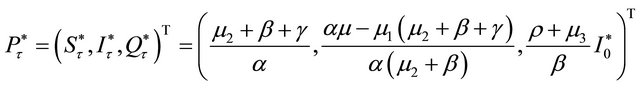
In the presence of infection , substituting in the system we obtain the second equilibrium point:
 (9)
(9)
Using the simplified and intuitive point theorem, Lyapunov square near the fixed point, and the solutions of the nonlinear system associated with the linear system by applying the Taylor formula of order 1.
Let

we note h, k, and m are the small perturbations. The formula for the Taylor series expansion.
We calculate the Jacobian matrix according to the system (3) with  The epidemic is locally asymptotically stable if and only if all eigenvaluesof the Jacobian matrix J have negative real part. The eigenvalues can be determined by solving the characteristic equation.
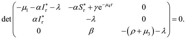 (10)
(10)
Since , we have
 . (11)
Then (10) is then written:
 . (12)
The caracteristic equation is as follow:
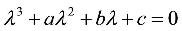 . (13)
with the notations:
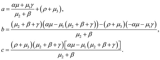
When  we have
  and
and  The real parts of eigenvalues are négative, then the equilibrium
  is locally asymptotically stable.
With , system (3) has a unique non-trivial equilibrium
  is locally asymptotically stable.
4. The Adomian Decomposition Method
The Adomian decomposition method has been applied to broad classes of problems in many fields such as mathematics, physics, biology. This method solves the functional equations of different types, and the advantage of this method is that it solves a problem at the direct scheme, the solution is obtained as a series sounds fast converging. We consider the operator equation , when
  is the operator represents a general nonlinear ordinary differential and
  is a given function. The linear part of
  can be decomposed into
 ,
,  is easily invertible and R is the remainder of F. It is therefore assumed that the nonlinear problem can be written as
 (14)
(14)
where  represents the nonlinear terms (
 is a nonlinear operator).
 : is invertible (L is the derivative highest for what is supposed to be invertible).
  is a linear differential operator (of the order of less than L) and
  is the source term.
It can be written
 (15)
(15)
Since L is invertible we also have
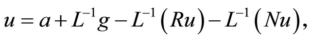 (16)
(16)
where  is the solution of the homogeneous equation
 , with initial conditions. The decomposition of the nonlinear term
 , and to do so, Adomian developed a very elegant technique as follows. We define the parameter
  decomposition, then
  is a function of
  next expansion
  Maclurian series from
 .
.
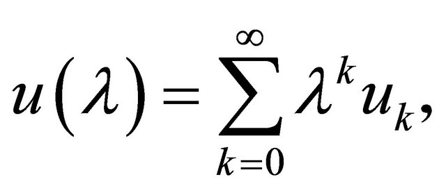
We have  in the form of a series,
 (17)
(17)
We decompose the nonlinear term,  as a series of special polynomials called Adomian polynomials,
 (18)
(18)
These polynomials are obtained by introducing a parameter  and writing,
 (19)
(19)
we deduce that
 (20)
(20)
we have:
 (21)
(21)
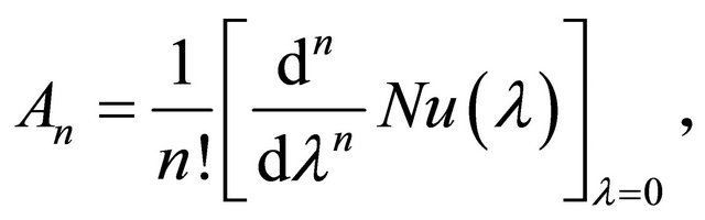
To determine the  we can use the following method,
 (22)
(22)
Then
 (23)
(23)
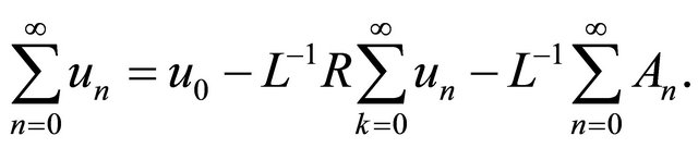
Finally a solution is given as
 (24)
(24)
The exact solution is
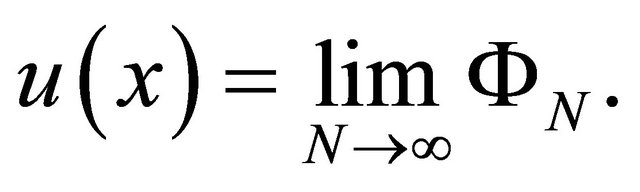 (25)
(25)
4.1. The Resolution to the System with Adomian Decomposition Method
It has a direct application of the Adomian decomposition method system. We note that the system is a more general homogeneous system of ordinary differential equations where the nonlinear term is the product of two variables. We consider the general form of a system of differential equations given as follows.
 (26)
(26)
We can write the system of equations above as operator with  is the first nonlinear term and
  the second term is linear,
  differential operator
 (27)
(27)
With applying the differential operator inverse  we have
 (28)
(28)
The solution  is given as
 (29)
(29)
The first nonlinear term is
 (30)
(30)
With applying the differential operator inverse  we have
 (31)
(31)
The first linear term is
 (32)
(32)
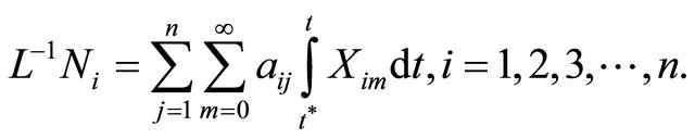
With applying the differential operator inverse  about the Equation (18) on obtient:
 (33)
(33)
For  we have
 (34)
(34)
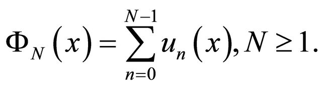
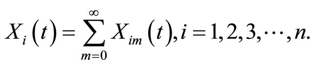
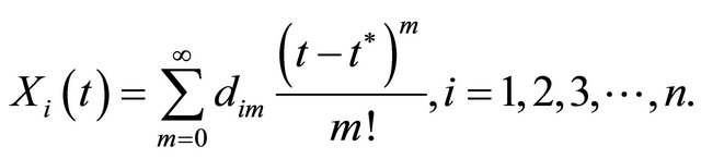
So if we write the solution for each  as follows
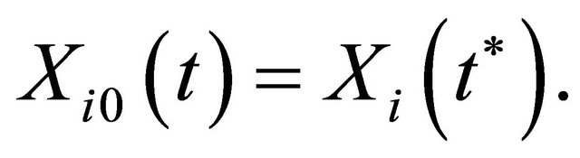 (35)
(35)
 (36)
(36)
 (37)
(37)

 (38)
(38)
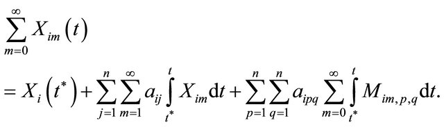
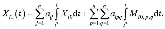
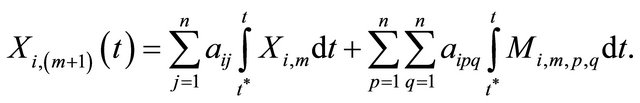
With applying the Adomian polynomial and then the general solution, is defined as follows 
 (39)
(39)
Solutions  are given as follows:
 (40)
(40)
 (41)
(41)
4.2. Solve the System Using the Method (MADM)
The solution explicite
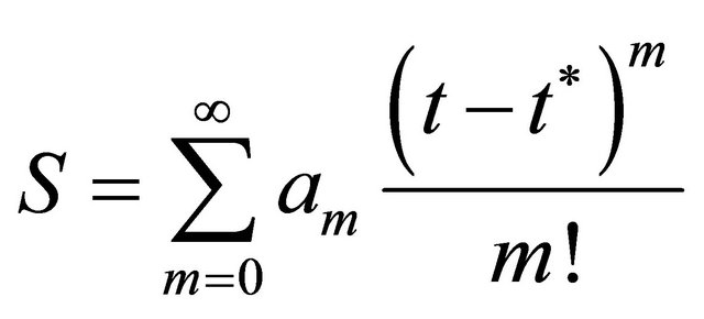 (42)
(42)
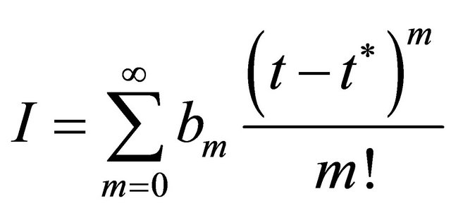 (43)
(43)
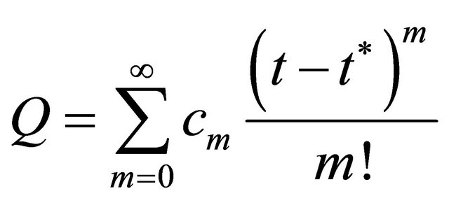 (44)
(44)
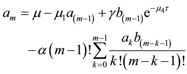
The coefficients are given with relations reccurence as follows
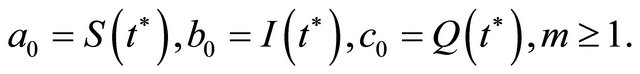 (45)
(45)
 (46)
(46)
 (47)
(47)
 (48)
(48)
5. Conclusion
This paper examined the asymptotic stability of the disease-free equilibrium and endemic equilibrium equation. If , we proved that the disease-free equilibrium is globally asymptotically stable for any delay time, and if
 , it was proved that the endemic equilibrium is zero, and disease-free equilibrium becomes unstable. We also derived two sufficient conditions for local asymptotic stability of the endemic equilibrium and sufficient condition for asymptotic stability. We resolve the system with the the adomian decompostion method.