Resonant Homoclinic Bifurcations with Orbit Flips and Inclination Flips ()
1. Introduction and Hypotheses
Flips homoclinic bifurcations are comprehensively investigated during the last decade (see [1-10]), which produce complicated bifurcations, such as the saddlenode bifurcations, the period-doubling bifurcations and the homoclinic-doubling bifurcations.
Recently, the flip of heterodimensional cycle or accompanied by transcritical bifurcation is discussed much (see [11-13]). The double and triple periodic orbit bifurcation are proved to exist, and also some coexistence conditions for homoclinic orbits and periodic orbits. But their research is not focused on multiple flips since it is a interesting problem and full of challenges due to the high codimension and complexity. In this paper, we develop a study of resonant homoclinic bifurcation with one orbit flip and two inclination flips, where the resonance takes place in the tangent direction of the homoclinic orbit. This is a codimension-4 problem, by using the local moving frame method established in [11,14,15], we get the existence of a double 1-periodic orbit, some 1-periodic orbits and 1-homoclinic orbits, and the coexistence conditions of 1-periodic orbits and 1-homoclinic orbits.
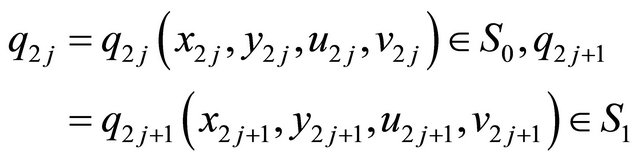
We consider the following two systems,
 (1.1)
(1.1)
 (1.2)
(1.2)
where 

 .
.
Notice that system (1.2) is an unperturbed system of (1.1) and assume it has an orbit
homoclinic to the hyperbolic equilibrium , which has two negative and two positive eigenvalues,
 , and
, and .
.
Hypotheses
Set  (resp.
 ) and
) and  (resp.
 ) the stable (resp. strong stable) manifold and unstable (resp. strong unstable) manifold of the equilibrium
 , respectively. We suppose that
(H1)  for
for , where
  and
and .
.
(H2) Define then
then  and
and  are unit eigenvectors corresponding to
  and
and  respectively, where
  is the tangent space of the corresponding manifold
  at the saddle
 , and the similar meaning for
 .
.
(H3) Denote by  and
and  the unit eigenvectors corresponding to
  and
and  respectively, there are

Remark 1.1 Hypotheses (H1) is a resonant condition, while (H2) - (H3) mean the homoclinic orbit has one orbit flip and two inclinations flips.
The paper is organized as follows. In Section 2, we first transform system (1.1) into two normal forms, then construct a regular map in some neighborhood of the homoclinic orbit and a singular map in some neighborhood of the equilibrium respectively to establish the Poincaré map. In Section 3, we develop the bifurcation study through searching for solutions of the bifurcation equation. Finally a short conclusion about the flips bifurcation is given in Section 4.
2. Local Active Coordinate Frame and Poincaré Map
We first give two normal forms of system (1.1) and then construct the Poincaré map. Firstly system (1.1) can be transformed into the following form in some neighborhood  of the origin
  due to the theory of invariance manifolds, (refer to [14,15])
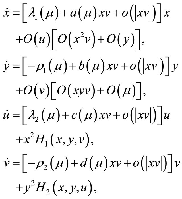 (2.1)
(2.1)
where 

 and
and .
.  and
and  are parameters depending on
 .
.
One may see that from (2.1),  and
and  are straightened locally to be the
  axes in neighborhood of
 , so it is possible to take some time
  large enough, such that
  and
and , where
  is small and
 .
.
Now consider the linear variational system
 (2.2)
(2.2)
and its adjoint system
 (2.3)
(2.3)
Matrix theory shows that system (2.2) has a fundamental solution matrix and furthermore it can be chosen as follows (refer to [11,14-15])
Lemma 2.1 There exists a fundamental solution matrix  of system (2.2) satisfying
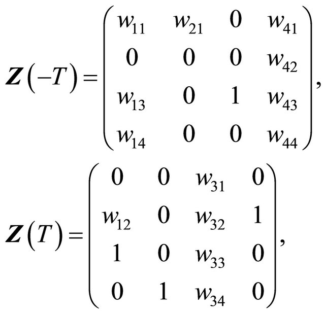
where

and , and
, and .
.
Obviously  is a fundamental solution matrix of system (2.3), denote by
 .
.
We here introduce a new coordinate  and set
 (2.4)
(2.4)
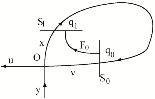
Naturally we can choose two cross sections of , see Figure 1,

Substitute (2.4) into (1.1), there is
Integrating both sides from  to
to , we further have
 (2.5)
(2.5)
where
 .
.
Equation (2.5) defines indeed a map  in some tube region near
 ,
,

see Figure 1(a). If set
 (a)
(a) (b)
(b)
Figure 1. Transition maps. (a) F1: S1→S0; (b) F0: S0→S1.
and
we can obtain the following expressions,
 (2.6)
(2.6)
 (2.7)
(2.7)
and
 (2.8)
(2.8)
Using the flow of system (2.1) in the neighborhood , we can set up a map

defined as (see [14,15])
 (2.9)
(2.9)
where  is the Silnikov time and
  is the time going from
  to
to , see Figure 1(b).
From the above the Poincaré map

is obtained
Then the corresponding associated successor function 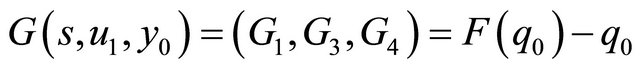 is
is
 (2.10)
Since  is defined by the flying time from the point in
  to
to , obviously
  means
means  is limited;
  means
means , which indicate the existence of a periodic orbit or a homoclinic orbit of system (1.1). So in the following section, we focus us on the solutions
  of (2.10).
3. Bifurcation Results
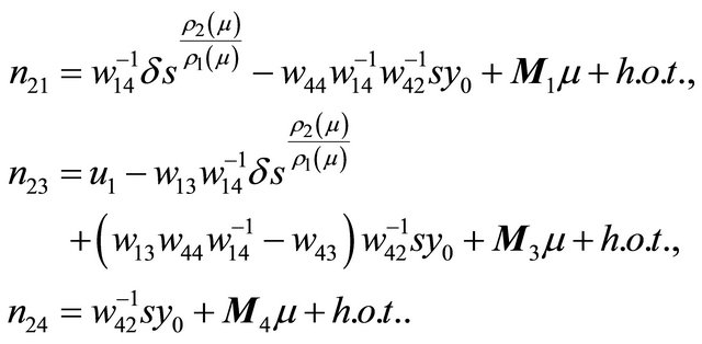
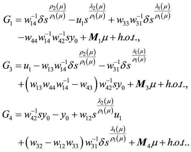
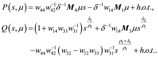
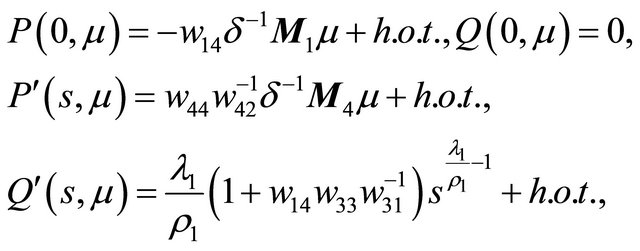
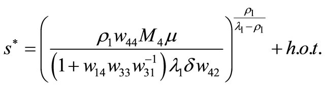
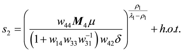
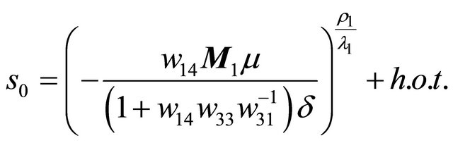
The last two equations in (2.10) give

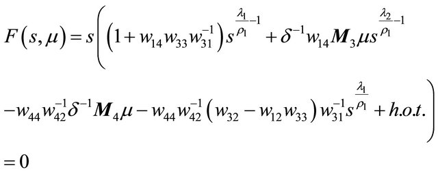
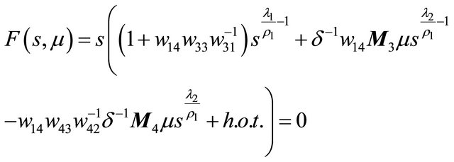
Then from  we get the bifurcation equation
 (3.1)
(3.1)
Notice that we have put higher orders terms into  and omitted the parameter
  in the eigenvalues for concision.
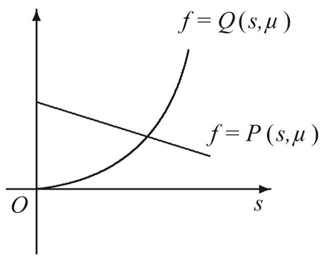
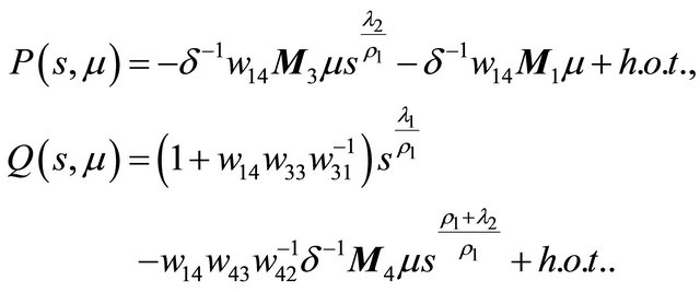
Define two functions as
Indeed here . By analysis of the curves
  and
and , one may immediately get the following statements.
Theorem 3.1 Suppose that , then in the region
 , system (1.1) has a unique 1-periodic orbit near
 ; in the region
 , system (1.1) has not any 1-periodic orbit.
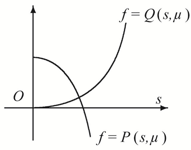
Proof Because
the curve  has no inflexion point, so th e line
  and the curve
  must intersect at a unique point in the region
 , where
and
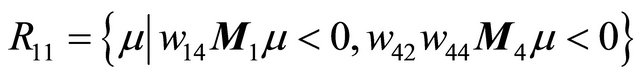
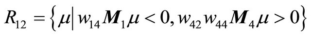 see Figure 2(a). Namely there exists a point
  such that
 therefore system (1.1) has a unique 1-periodic orbit. On the contrary, there is not such a intersection point in the region
 see Figure 2(b).
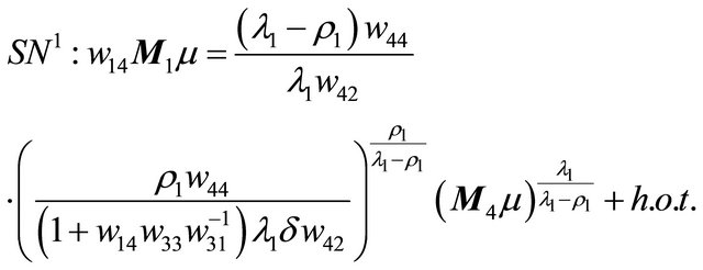
Theorem 3.2 Suppose that , then in the region
 , system (1.1) has a unique double 1- periodic orbit near
  located in the bifurcation surface
 .
.
Moreover when  lies on the side of
  pointing to the (resp. opposite) direction
 , system (1.1) has two (resp. not any) 1-periodic orbits near
 .
.
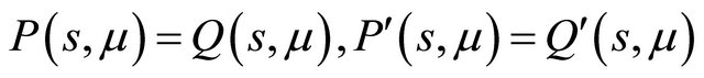
Proof We know that the existence of a double 1-periodic orbit corresponds to a double solution  of (3.1). According to the proof of Theorem 3.1, it is enough to search the tangent point of the curves
  and
and
 (a)
(a) (b)
(b)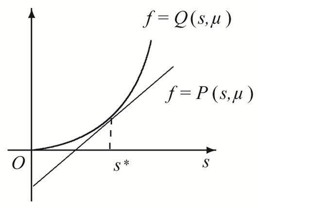 (c)
(c)
Figure 2. Location between the curves. (a) μ ∈ R11∪R12; (b) μ ∈ R21; (c) μ ∈ R22.
 , that is to solve
and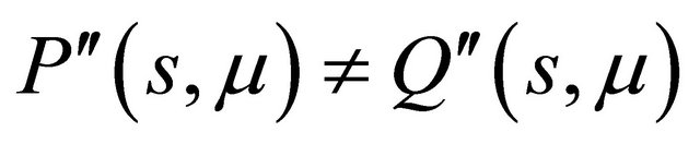 , concretely,
 (3.2)
(3.2)
Then the tangent point
as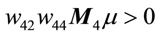 . Combining the first equation of (3.2) with the tangent point, we obtain the double periodic orbit bifurcation surface
in the region . At the same time, when
 , the line
  lies under the curve
 , see Figure 2(c), so if
  increases, the line must intersects the curve at two sufficiently small positive points, therefore system (1.1) undergos two 1-periodic orbits. Then the proof is complete.
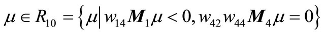
Theorem 3.3 Suppose that , then system (1.1) has only one 1-homoclinic orbit near
  in the region
 ; has only one 1-periodic orbit near
  in the region
 ; has exactly one 1-homoclinic orbit and one 1-periodic orbit near
  in the region
 ; has not any 1-periodic orbit or 1-homoclinic orbit in the region
 .
.
Proof When
 ,
,
has always two solutions  and
and
or has only a zero solution  for
for
 .
.
While for
 apparently the line
  is horizontal. So
  gives merely a solution
 .
.
The last conclusion is obvious for
 .
.
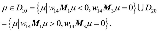
In the following, we study the case . Then (3.1) is

Similar to the proof of Theorem 3.1 and 3.3, we have Theorem 3.4 Suppose that , then in the region
 , system (1.1) has a unique 1-periodic orbit near
 ; in the region
 , system (1.1) has not any 1-periodic orbit.
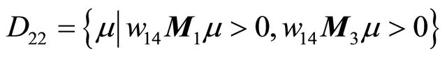
Proof Redefine
By studying the relationship between the curves  and
and , it is easy to get the main ideas, see Figure 3. Here
 (a)
(a) (b)
(b)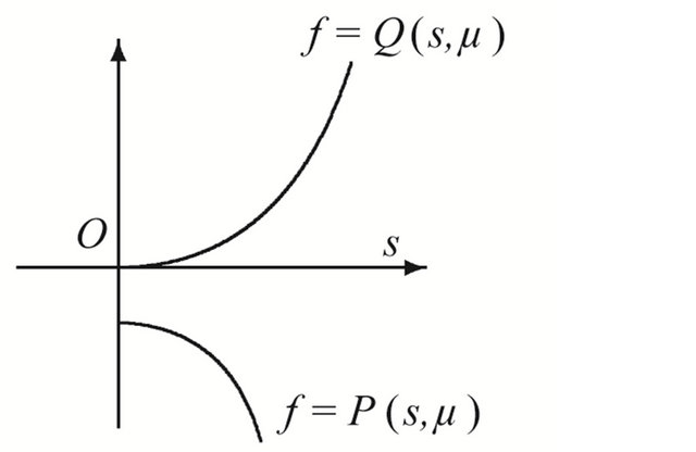 (c)
(c)
Figure 3. Location between the curves. (a) μ ∈ D12; (b) μ ∈ D21; (c) μ ∈ D22.
and
 .
.
Remark 3.1 For the case , system (1.1) has no longer double 1-periodic orbits and the double 1-periodic orbit bifurcation surfaces.
Theorem 3.5 Suppose that , then system (1.1) has only one 1-homoclinic orbit near
  in the region
 ; has only one 1-periodic orbit near
  in the region
 ; has not any 1-periodic orbit or 1-homoclinic orbit in the region
 .
.
Proof Notice that
has only a zero solution  for
for
 .
.
And the line  is horizontal for
Thereby the conclusion is clear. We omit the details here.
4. Conclusion
The theoretical development of flip bifurcations indeed advanced much in recent years. More and more complicated cases with several flips or accompanied by transcritical bifurcation nowadays are discussed. This paper focuses on a kind of three flips homoclinic case with resonance and introduces an effective method to extend the study. By the analysis of the bifurcation equation, the existence of a double 1-periodic orbit, some 1-periodic orbits and 1-homoclinic orbits, and the coexistence conditions of 1-periodic orbits and 1-homoclinic orbits are given. From the study, one notice that different leading terms of the bifurcation equation may cause different bifurcation phenomena, so we can go further in the future work.
[16] NOTES