Some Exact Results for an Asset Pricing Test Based on the Average F Distribution ()
1. Introduction
The idea of the average F test was first introduced to the literature by [1] as a means of testing asset pricing theories in linear factor models. Recently [2] developed the idea further by focusing on the average pricing error, extending the multivariate F test of [3]. They show that the average F test can be applied to thousands of individual stocks rather than a smaller number of portfolios and thus does not suffer from the information loss or the data snooping biases. In addition, the test is robust to ellipticity. More importantly, [2] demonstrate that the power of average F test continues to increase as the number of stocks increases.
One drawback of the average F test is that [2] did not provide the closed form solution for the average F density function. Despite the fact that the average F statistic has been used in other areas of econometrics, e.g., [4] in the study of structural breaks of unknown timing in regression models, the functional form of the average F distribution remains unknown.
In this study we propose a few analytical developments for the average F distribution. Although the complete functional form is not provided, our results might be useful toward further research in the future.
2. Definition of the Average F Distribution
A testable version of linear factor models is
 (1)
(1)
where  is a
is a  vector of excess returns for
  assets and
  is a
is a  vector of factor portfolio returns,
  is a vector of intercepts,
  is an
is an  matrix of factor sensitivities, and
 is a
is a  vector of idiosyncratic errorswhose covariance matrix is
 . For the null hypothesis
  tested against the alternative hypothesis
 , the average
  -test statistic is defined as
 (2)
(2)
where

and  and
and  are the maximum likelihood estimators of
  and
and , respectively. Under the classical assumption that asset returns are multivariate normal conditional on factors, the average F statistic is distributed as
 (3)
(3)
where  is a
is a  statistic with 1 degree of freedom in the numerator and
  degrees of freedom in the denominator.
3. Characteristic Function of the Average F Distribution
The distribution function of the average  statistic is unknown. Note that all
  -distributions in Equation (3) have the same degrees of freedom, and
  is thus distributed as the sample mean of
  independent and identically distributed
  distributions. Let
  be a variable distributed as
 , where
 , and denote its probability density function as
 . Then the characteristic function of the
  distribution can be derived as follows
 (4)
(4)
Let  and
and , then
 (5)
(5)
where  is the gamma function,
  is the imaginary number, and
  is Tricomi’s confluent hypergeometric function. Equation (5) was first formulated by [5]. Tricomi’s confluent hypergeometric function is
 (6)
(6)
where  is Kummer’s confluent hypergeometric function which is defined as
 (7)
(7)
See [6] for a detailed explanation of various types of hypergeometric functions and their applications to economic theory.
If b in Equation (7) is a non-positive integer,  and thus

is not defined. Note that  is a positive integer as it represents the degrees of freedom in the denominator of the
  distribution; thus, we need
 and
and 
in Equation (6) to be positive integers. However, since n is a positive integer, both
 and
and 
cannot be kept to be positive integers. More generallywhen 
we have a definition referred to as the “logarithmic case” alternative to Tricomi’s confluent hypergeometric function in (6). See [6] and [7] (Vol. 1, pp. 260-262 and Vol. 2, p. 9) for discussions on the logarithmic case.
Let  be defined as the characteristic function of the
  independent
  variable. Then, the characteristic function of
  is
is
 (8)
(8)
where  is defined in (5). Therefore, the density function of the average F statistic
 ,
,  , under the null hypothesis is obtained by the following;
 (9)
(9)
where y is a variable distributed as the average of the  different
  distributions
 This mean of F-distributions can be used when the variance-covariance matrix
  is a diagonal matrix.
4. The Exact Distribution of Average F Test for Small N
When , we have
  Using the result that
  is the square of
 , i.e., a
  distribution with
  degrees of freedom, we see that the
  of
of  is given by
 , letting
 ,
,
 (10)
(10)
where the  of
of  can be found in [8].
To find the  of
of  when
when ,
,  , we proceed as follows. Let
  be the associated random variable, and
  and
and  be the two independent
  variables. Then we have
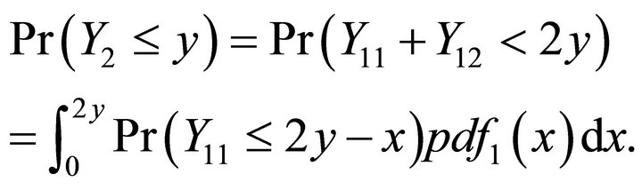
Therefore 
where  is given by Equation (10). More generally, by induction, it follows that
 (11)
(11)
Although it is hard to make much progress with Equation (11) in obtaining closed form solutions, we note the following. From known moments of the  distribution, it is possible to calculate the moments of
  for any
 , where they exist.
Proposition 1. The moments of S exist for
 .
.
Proof. Let  Then
Then 
so that the highest order term, for any , is
, is  Now from Equation (10),
 and thus
 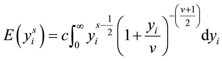 which exists if
Proposition 2 For ,
,  can be represented as a scale Beta type II function.
Proof. For  given by Equation (10), let

Then  and simple change of variable shows that
  is a Beta
  random variable.
Since Proposition 2 establishes that  is a scaled Beta, we now have a representation of
  Denoting
  to reflect the dependence on
 , it follows from Proposition 2 that
 (12)
(12)
where  denotes a type II beta with parameters
  and
and  and the
  outside
 reflects the scale factors. Thus Equation (12) establishes that
  can be represented as a linear combination of Beta type II distributions.
The literature on density functions of linear combination of Beta distributions is rather sparse. [9] present expressions for linear combinations of Beta distributions when . Thus using their results we can arrive at an expression for
  which is complex and depends upon hypergeometric functions. Extensions for
  do not appear to be derived as yet.
5. Conclusion
We provide some developments on the average F test distribution. Although simulation of the statistic is straightforward, an understanding of the functional form is invaluable in terms of appreciation of the properties of the test statistic. We leave a full solution of the problem for future study.