The First Order Autoregressive Model with Coefficient Contains Non-Negative Random Elements: Simulation and Esimation ()
1. Introduction
It is well-known that many time series in finance such as stock returns exhibit leptokurtosis, time-varying volatility and volatility clusters. The generalized autoregressive conditional heteroscedasticity (GARCH) and the random coefficient autoregressive (RCA) model have been caturing three characteristics of financial returns.
The RCA models have been studied by several authors [1-3]. Most of their theoreic properties are well-known, including conditions for the existence and the uniqueness of a stationary solution, or for the existence of moments for the stationary distribution. In this paper, we address the stationary conditions for the RCA model, the existence and the uniqueness of a stationary solution and parameter estimation problem for the RCA model with the coefficient have a non-negative random elements.
2. Stationary Conditions of the Series
Consider time series  satisfying
 (1)
(1)
where 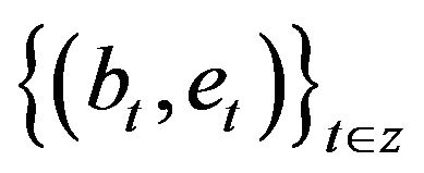 are random vectors with independent identical distribution defined in a certain
  probability space(2)
Firstly, we consider the property of the stochastic variable
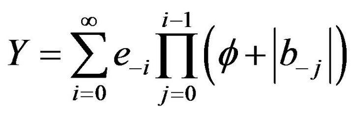 (3)
(3)
Let .
.
Lemma 1. Suppose that condition (2) satisfied,
 (4)
(4)
If
 (5)
(5)
Y determined by (3) will be absolute convergence with probability 1.
Proof.
Assume , according to the law of great numbers, existing stochastic variable
  such that:
 (6)
(6)
where . Then
 (7)
(7)
We will prove . Indeed, due to
 and in accordance with lemma Borel-Cantelli, sufficient condition here means proving
 with
with  We have:

From (7), we have .
.
If , (6) can always correct with some
 . Therefore, (7) is always true.
Lemma 2. Suppose that (2) and (5) meet
 with some
 . Then, existing
  such that
 .
.
Proof.
Suppose 
We have , and owing to
 ,
,  is a decreasing function in the neighborhood of 0. Hence, existing
  such that
 . Generally less, suppose that
  Due to the convex, we have
  với
với .
.

Use condition (2) and , we obtain:

Lemma 3. Assume (2) and (5) are satisfied with
 . Then
 .
.
Proof.
Due to condition (2) and inequality Minkowski
 . Hence,
 .
.
Theorem 1: Suppose that (1), (4) and (5) satisfied with the almost sure convergence of
 and process
  is the stationary solution of (1)
Proof.
 is convergent absolutely, acording to Lemma 1 We have:
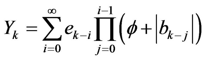 . Therefore:

 is the single solution of (1)
Obviously,  is a stationary series and
  is independent of
 .
.
3. Estimation of Model Parameters
Suppose that

In this section, we care about estimating vectors of  based on Quasi-Maximum Likelihood method.
With , we have:

but , so
, so

Therefore, we have following likelihood function

Maximum likelihood estimators determined by:
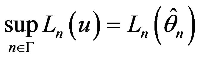 (8)
(8)
where  is a certain optional appropriate area of
Let

Then (8) can be written as 
Assume
 (9)
(9)
Now, the consistence of maximum livelihood estimates  is said.
Theorem 2. Suppose (2), (4), (5), (8), (9) satisfied and . We have
 .
.
Proof.
Let

and 
We will prove  be continuous on
 .
.
Indeed,
On the other hand,

But


Then

 is a continuous function in acordance with
 . Next, we will prove:
 .
.
In fact,
where

and  if and only if

If
 If
If  or
or ,
, 
But 
But  is a stationary series

But , take conditional expectations
  in both sides, we have:

But 
Return to theorem , so
, so

But series  is stationary and ergodic with
 , according to Ergodic theorem, we have:

With each positive integer  is a continuous function in compact set G, so

Let  -compact set in
  with positive distance to
 . Owing to g1(u) being continuous in
 , existing an open sphere U(u) with center u with
  such that:
 .
.
Sets  are open covers of C, so C holds such finite open covers, are called
  of C. In accordance with Ergodic thoerem, with every
 , we have:

See that

In out of events  with
with  with
with  satisfying:
 .
.
Therefore, 
But  is continuous and
  is singly minimum of

Let U is a open sphere with center  and enough small radius and
 . If
. If , existing a random subseries
  such that with
 , we have:

But 
hence, with each above , existing random variable
  such that
This completes the proof. 
4. Simulation
In this section, we simulate series (1) with different values of . These simulations show stationary and non-stationary series cases.
We simulate series (1) with different values of  and in each case we can check the stationary conditions of the series (1) by Lemma 1. In Figure 1, we see that the series is not stationary with the negagtive slope
  and in Figures 2 and 3 we simulate the not stationary series with positive slope
  and
and . Figure 4 presents a stationary but clustering series, Figures 5-7 present stationary series with parameters are
 ,
,  and
and .
.

Figure 1. Simulation for series Yt defined by (1) with .
.

Figure 2. Simulation for series Yt defined by (1) with .
.
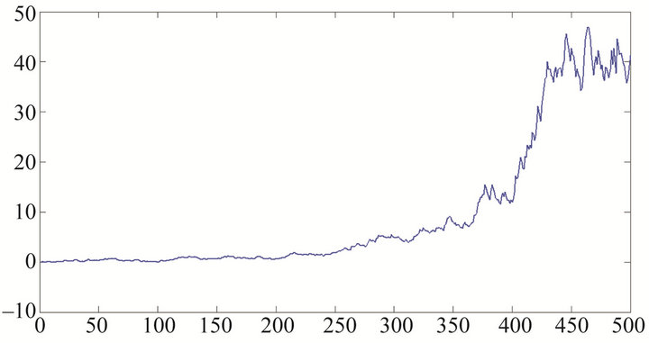
Figure 3. Simulation for series Yt defined by (1) with .
.

Figure 4. Simulation for series Yt defined by (1) with .
.

Figure 5. Simulation for series Yt defined by (1) with .
.
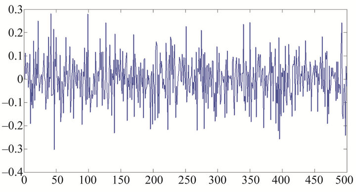
Figure 6. Simulation for series Yt defined by (1) with .
.

Figure 7. Simulation for series Yt defined by (1) with .
.
5. Application for Real-Time Series
In this section, we use model (1) for the model of return series of the price of gold on the free market in Hanoi, Vietnam. Figure 8 show the Return series of Gold price .
.
From the data series we estimate for vector
 is
is . So, we can use the following model to forecast the future value of gold price:
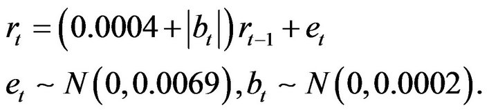

Figure 8. Return series of Gold price rt.

Figure 9. Simulation for series Yt defined by (1) with .
.
Figure 9 below is a simulation of the process (1) with parameters .
.