Modified Piyavskii’s Global One-Dimensional Optimization of a Differentiable Function ()
1. Introduction
We consider the following general global optimization problems for a function defined on a compact set 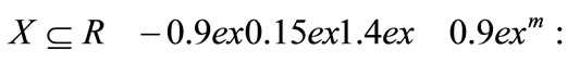
(P) Find

such that

(P1) Find  such that fopt = f(xopt) ≥ f* − ε, where ε is a small positive constant.
Many recent papers and books propose several approaches for the numerical resolution of the problem (P) and give a classification of the problems and their methods of resolution. For instance, the book of Horst and Tuy [1] provides a general discussion concerning deterministic algorithms. Piyavskii [2,3] proposes a deterministic sequential method which solves (P) by iteratively constructing an upper bounding function F of f and evaluating f at a point where F reaches its maximum, Shubert [4], Basso [5,6], Schoen [7], Shen and Zhu [8] and Horst and Tuy [9] give a special aspect of its application by examples involving functions satisfying a Lipschitz condition and propose other formulations of the Piyavskii’s algorithm, Sergeyev [10] use a smooth auxiliary functions for an upper bounding function, Jones et al. [11] consider a global optimization without the Lipschitz constant. Multidimensional extensions are proposed by Danilin and Piyavskii [12], Mayne and Polak [13], Mladineo [14] and Meewella and Mayne [15], Evtushenko [16], Galperin [17] and Hansen, Jaumard and Lu [18,19] propose other algorithms for the problem (P) or its multidimensional case extension. Hansen and Jaumard [20] summarize and discuss the algorithms proposed in the literature and present them in a simplified and uniform way in a high-level computer language. Another aspect of the application of Piyavskii’s algorithm has been developed by Brent [21], the requirement is that the function is defined on a compact interval, with a bounded second derivative. Jacobsen and Torabi [22] assume that the differentiable function is the sum of a convex and concave functions. Recently, a multivariate extension is proposed by Breiman and Cutler [23] which use the Taylor development of f to build an upper bounding function of f. Baritompa and Cutler [24] give a variation and an acceleration of the Breiman and Cutler’s method. In this paper, we suggest a modified Piyavskii’s sequential algorithm which maximizes a univariate differentiable function f. The theoretical study of the number of iterations of Piyavskii’s algorithm was initiated by Danilin [25]. Danilin’s result was improved by Hansen, Jaumard and Lu [26]. In the same way, we develop a reference algorithm in order to study the relationship between nB and nref where nB denotes the number of iterations used by the modified Piyavskii’s algorithm to obtain an ε-optimal value, and nref denotes the number of iterations used by a reference algorithm to find an upper bounding function, whose maximum is within ε of the maximum of f. Our main result is that nB ≤ 4nref + 1. The last purpose of this paper is to derive bounds for nref. Lower and upper bounds for nref are obtained as functions of f(x), ε, M1 and M0 where M0 is a constant defined by

and M1 ≥ M0 is an evaluation of M0.
2. Upper Bounding Piecewise Concave Function
Theorem 1. Let
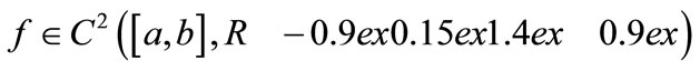
and suppose that there is a positive constant M such that
 (1)
(1)
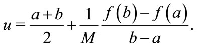
Let

and

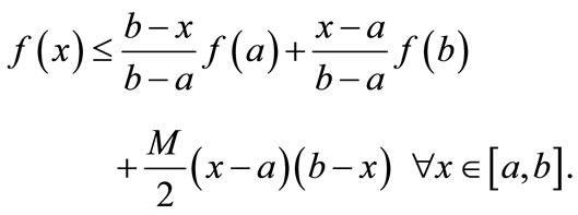
Then

Proof. Let

we have

Then Ψ is a concave function, the minimum of Ψ over [a, b] occurs at a or b. Then

for all .
.
This proves the theorem.
Remark 1. Let
Then the maximum Φ* of Φ(x) is:

If the function f is not differentiable, we generalize the above result by the following one:
Theorem 2. Let f be a continuous on [a, b] and suppose that there is a positive constant M such that for every h > 0
 (2)
(2)
Then
Proof. without loss of generality, we assume that f(a) = f(b) = 0 and M = 0.
Let us consider the function f(x) − Φ(x) instead of the function f(x). It suffice to prove that
Suppose by contradiction that f* > 0, and let
The function f is continuous, f(u) = f* > 0, thus a < u < b, consequently  for h > 0 small and we have f(u − h) ≤ f(u) and f(u + h) < f(u).
Since M = 0, this contradicts the hypothesis (3). Hence f* ≤ 0.
Remark 2. Since the above algorithm is based entirely on the result of Theorem 1, it is clear that the same algorithm will be adopted for functions satisfying condition (2).
If f is twice continuously differentiable, the conditions (1) and (2) are equivalents.
3. Modified Piyavskii’s Algorithm
We call subproblem the set of information

describing the bounding concave function


The algorithm that we propose memorizes all the subproblems and, in particular, stores the maximum  of each bounding concave function Φi over [ai, bi] in a structure called Heap. A Heap is a data structure that allows an access to the maximum of the k values that it stores in constant time and is updated in O(Log2k) time. In the following discussion, we denote the Heap by H.
Modified Piyavskii’s algorithm can be described as follows:
3.1. Step 1 (Initialization)
• k ← 0
• [a0, b0] ←[a, b]
• Compute f(a0) and f(b0)
• 
• 
• Let  be an upper bounding function of f over [a0, b0]
• Compute 
• 
• if  Stop,
Stop,  is an ε-optimal value

3.2. Current Step (k = 1, 2, ···)
While H is no empty do
• k ← k + 1
• Extract from H the subproblem 
with the largest upper bound 
• 

3.2.1 Update of the Best Current Solution
for j = l, k do
3.2.1.1. Lower Bound
If  then
then


Else

End if
3.2.1.2. Upper Bound
• Build an upper bounding function Φj on [aj, bj]
• Compute 
• Add  to H
to H
End for
• Delete from H all subproblems
with 
3.2.2. Optimality Test
• Let  be the maximum of all
• If  then Stop,
  is an ε-optimal value
End While
Let [an, bn] denote the smallest subinterval of [a, b] containing xn, whose end points are evaluation points. Then the partial upper bounding function Φn−1(x) spanning [an, bn] is deleted and replaced by two partial upper bounding functions, the first one spanning [an, xn] denoted by Φnl(x) and the second one spanning [xn, bn] denoted by Φnr(x) (Figure 1).
Proposition 1. For n ≥ 2 the upper bounding function Φn(x) is easily deduced from  as follows:

and

Proof. In the case where


Figure 1. Upper bounding piece-wise concave function.
is in [an, xn], then from remark 1, the maximum of  is given as follows
 (3)
(3)
The maximum of  spanning [an, bn] is reached at the point

We deduce that

then

By substitution in expression (3), we have the result. We show in the same way that the maximum  of
of  defined in [xn, bn] is given by:

Remark 3. Modified Piyavskii’s algorithm obtains an upper bound on f within ε of the maximum value of f(x) when the gap  is not larger than ε, where

But f* and

are unknown. So modified Piyavskii’s algorithm stops only after a solution of value within ε of the upper bound has been found, i.e., when the error  is not larger than ε. The number of iterations needed to satisfy each of these conditions is studied below.
4. Convergence of the Algorithm
We now study the error and the gap of Φn in modified Piyavskii’s algorithm as a function of the number n of iterations. The following proposition shows how they decrease when the number of iterations increases and provides also a relationship between them.
Proposition 2. Let  and
and  denote respectively the error and the gap after n iterations of modified Piyavskii's algorithm. Then, for
  1)
1)  2)
2)  3)
3) 
Proof. First, notice that  and
and  are non increasing sequences and
  is nondecreasing. After n iterations of the modified Piyavskii's algorithm, the upper bounding piece-wise concave function
  contains
  partial upper bounding concave functions, which we call first generation function. We call the partial upper bounding concave functions obtained by splitting these second generation function.
  must belong to the second generation for the first time after no more than another
  iterations of the modified Piyavskii’s algorithm, at iteration m (m ≤ 2n − 1).
Let k  be the iteration after which the maximum
  of
of  has been obtained, by splitting the maximum
  of
of  Then, in the case where

is in  and from proposition 1, we get:

where

and  is one of the endpoints of the interval over which the function
  is defined.
1) We have

where

If  therefore, we have

If  we will consider two cases:
• case 1
If  then
then  and if
  then
then  and the algorithm stops.
• case 2
 then we have

hence

(proposition 1).
Moreover

We deduce from these two inequalities that

Therefore

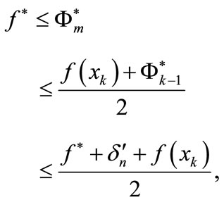
2) We have

We follow the same steps to prove the second point of 1) and show that 
3)
• case 1
If  or
or  then
then  and the algorithm stops.
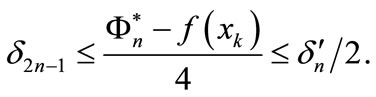
• case 2  First, we have

and
therefore  Hence
Hence
This proves the proposition.
Proposition 3. Modified Piyavskii’s algorithm (with ) is convergent, i.e. either it terminates in a finite number of iterations or

Proof. This is an immediate consequence of the definition of  and i) of proposition 2.
5. Reference Algorithm
Since the number of necessary function evaluations for solving problem (P) measures the efficiency of a method, Danilin [25] and Hansen, Jaumard and Lu [26] suggested studying the minimum number of evaluation points required to obtain a guaranteed solution of problem (P) where the functions involved are Lipschitz-Continuous on 
In the same way, we propose to study the minimum number of evaluation points required to obtain a guaranteed solution of problem (P) where the functions involved satisfy the condition (1).
For a given tolerance  and constant M this can be done by constructing a reference bounding piece-wise concave function
  such that
 with a smallest possible number
  of evaluations points
  in
in 
Such a reference bounding piece-wise concave function is constructed with  which is assumed to be known. It is of course, designed not to solve problem (P) from the outset, but rather to give a reference number of necessary evaluation points in order to study the efficiency of other algorithms. It is easy to see that a reference bounding function
  can be obtained in the following way:
Description of the Reference Algorithm
1). Initialization
• 
•  root of the equation

2). Reference bounding function
While  do
do
• compute 
• 
•  root of the equation

• 
End While.
3). Minimum number of evaluations points
• 
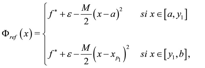
A reference bounding function  is then defined as follows (see Figure 2)

6. Estimation of the Efficiency of the Modified Piyavskii’s Algorithm
Proposition 4. For a given a tolerance  let
let  be a reference bounding function with
  evaluations points
  and
and  Let
Let  be a bounding function obtained by the modified Piyavskii’s algorithm with evaluation points
  where nC is the smallest number of iterations such that

Then we have
 (4)
(4)
and the bound is sharp for all values of 
Proof. The proof is by induction on  We initialize the induction at
• Case 1  (see Figure 3)
We have to show that  We have
and 
But 
hence

Therefore

hence the result holds.
• case 2 y1 < b. (see Figure 4)
If nc = 2, (4) holds. In this case, we have
where

Assuming that  and
and  ( the proof is similar for
 ). We denote by
  and
and  the partial bounding functions defined respectively on
  and
and  and by
  a maximum value of
  We show that

and that  Indeed, we have

and

thus

If

is in  then
then
As

(see the proof of proposition 2), we have

If  then
then 
If  ≤ x3 then
  and (4) holds.
Assume now that (4) holds for  and consider nref = k + 1. The relation (4) holds for nc = 2, therefore we may assume that

If we let

the modified Piyavskii’s algorithm has to be implemented on two subintervals [x1, x3] and [x3, x2] There are two cases which need to be discussed separately:
• case 1 (see Figure 5)
There is a subinterval containing all the nref evaluation points of the best bounding function  Without loss of generality, we may assume that
  contains all nref evaluation points of
 . Let
. Let  and
and  be the solution of
  By symmetry, we have

Let  be the abscissa of the maximum of the last partial bounding function of
  Due to our assumption, we have

since otherwise there is an another evaluation point of f on the interval
Let  be the abscissa of the maximum of the partial bounding function of
  preceding
  In this case, we have

But  implies that nref = 1, which is not the case according to the assumption (nref ≥ 2). Therefore, this case will never exist.

Figure 5. The subinterval contains all the nref evaluation points.
• case 2 None of the subintervals contains all the nref evaluation points of Φref(x). We can then apply induction, reasoning on the subintervals [x1, x3] and [x3, x2] obtained by modified Piyavskii’s algorithm. If they contain  and
and  evaluation points respectively, [x1, x2] contains
  evaluation points as x3 belongs to both subintervals. Then (4) follows by induction on nref.
Consider the function f(x) = x defined on [0, 1], the constant M is equal to 4. For ε = 0 we have nC = nref + 1 (see Figure 6), and the bound (4) is sharp.
As noticed in remark 3, the modified Piyavskii’s algorithm does not necessarily stop as soon as a cover is found as described in proposition 4, but only when the error does not exceed ε. We now study the number of evaluation points necessary for this to happen.
Proposition 5. For a given tolerance ε, let nref be the number of evaluation points in a reference bounding function of f and nB the number of iterations after which the modified Piyavskii’s algorithm stops. We then have
 (5)
(5)
Proof. Let  Due to proposition 4, after
  iterations, we have
  Due to 3) of proposition 2, after
  iterations, we have

which shows that the termination of modified Piyavskii’s algorithm is satisfied. This proves (5).
7. Bounds on the Number of Evaluation Points
In the previous section, we compared the number of evaluation functions in the modified Piyavskii’s algorithm and in the reference algorithm. We now evaluate the number nB of evaluation functions of the modified Piyavskii’s algorithm itself. To achieve this, we derive bounds on nref, from which bounds on nB are readily obtained using the relation nref ≤ nB ≤ 4nref + 1.
Proposition 6. Let f be a C2 function defined on the interval [a, b]. Set
and let

Then the number nref of evaluation points in a reference cover Φref using the constant M1 ≥ M2 is bounded by the following inequalities:
 (6)
(6)

Figure 6. None of the subintervals contains all the nref evaluation points.
 (7)
(7)
Proof. We suppose that the reference cover Φref has nref − 1 partial upper bounding functions defined by the evaluation points

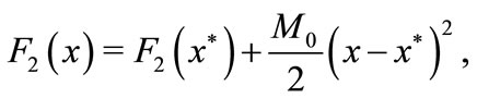
We consider an arbitrary partial upper bounding function and the corresponding subinterval [yi, yi + 1] fori i = 1, ···, nref − 1. To simplify, we move the origin to the point (yi, f(yi)). Let d = yi + 1 − yi , z = f(yi + 1) − f(yi) and h = f* + ε. We assume z ≥ 0 (See Figure 7).
Let  be the partial upper bounding function defined on [yi, yi + 1] and
  the point where

is reached, then

We deduce that

Let g1 be the function defined on [yi, yi + 1] by:

We have

Thus we have

Consider the function
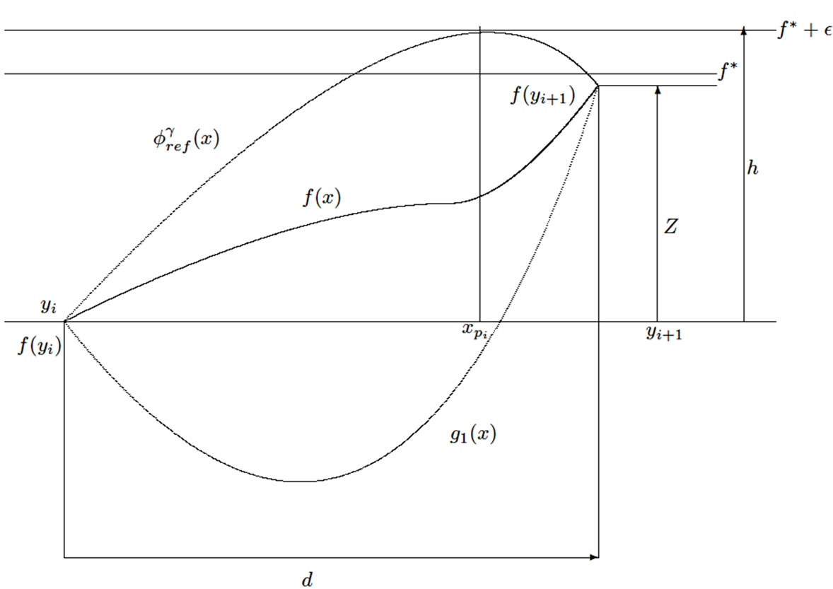
Figure 7. The reference cover Φref has nref − 1 partial upper bounding functions.

Let x1 and x2 be the roots of the equation F1(x) = 0; they are given by

Then F1 is written in the following way

Let


We have

Since θ ≥ 0 and g1 reaches its minimum at the point θ, then

and

Since

and

then

and

This proves (6).
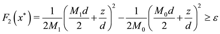
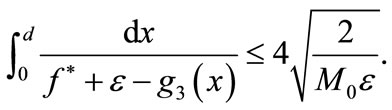
Now let us consider the function G defined and continuous on [yi, yi + 1] such that
• 
• 
Two cases are considered case 1: If
 (8)
(8)
then, the function G is given by

Hence

We consider
its derivative is

Thus F2 is expressed as follows
hence

Since
and 
then 
and

Moreover, the inequality
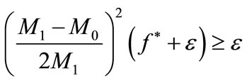
implies (8), this proves the first inequality of (7).
Case 2: Suppose that:
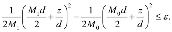 (9)
(9)
Let X1 et X2 be the roots of the equation

X1 and X2 are given by
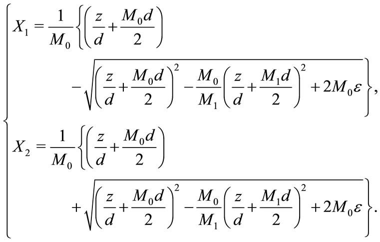
In this case, G is given by

We have

Moreover, M0 = M1 implies the condition (9) and we have

Therefore


and
Hence


Table 1. Computational results with  .
.

Table 2. The number of function evaluations of modified Piyavskii's algorithm for different values of ε and M.
8. Computational Experiences
In this section, we report the results of computational experiences performed on fourteen test functions (see Tables 1 and 2). Most of these functions are test functions drawn from the Lipschitz optimization literature (see Hansen and Jaumard [20]).
The performance of the Modified Piyavskii’s algorithm is measured in terms of NC, the number of function evaluations. The number of function evaluations NC is compared with (nref), the number of function evaluations required by the reference sequential algorithm. We observe that NC is on the average only 1.35 larger than (nref). More precisely, we have the following estimation
 .
.
For the first three test functions, we observe that the influence of the parameter M is not very important, since the number of function evaluations increase appreciably for a same precision ε.
NOTES