A New Full-NT-Step Infeasible Interior-Point Algorithm for SDP Based on a Specific Kernel Function ()
1. Introduction
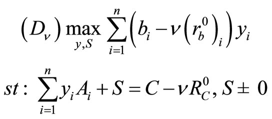
In this paper we deal with SDP problems, whose primal and dual forms are:

and

where ,
, . The matrices
 ,
,  are assumed to be linearly independent.
The use of Interior-Point Methods (IPMs) based on the kernel functions becomes more desirable because of the efficiency from a computational point of view. Many researchers have been attracted by the Primal-Dual IPMs for SDP. For a comprehensive study, the reader is referred to Klerk [1], Roos [2] and Wolkowicz et al. [3]. Bai et al. [4] introduced a new class of so-called eligible kernel functions for Linear Optimization (LO) which are defined by some simple properties following the same way of Peng et al. who have designed a class of IPMs based on a so-called self-regular proximities [5]. These methods use the new search directions which are different than the classic Newton directions. Some extensions were successfully made by Mansouri and Roos [6], Liu and Sun [7]. In the current paper, we propose a new infeasible interior-point algorithm, whose feasibility step is induced by a specific kernel function.
In the sequel, we denotes e as the all one vector and  the vector of eigenvalues of
 . Two different forms of norm will be used

2. The Statement of the Algorithm
We start usually with assuming that the initial iterates  and
and  are as follows

where I is the  identity matrix,
  is the initial dual gap and
  is such that

for some optimal solution  of
of  and
and .
.
2.1. The Feasible SDP Problem
The perturbed KKT condition for  and
and  is
is

Based on different symmetrization schemes, several search directions have been proposed.
As in Mansouri and Roos [6], we use in this paper, the so-called NT-direction determined by the following system
 (1)
(1)
where
 (2)
(2)
We also define the square root matrix .
.
The matrix D can be used to rescale X and S to be the same matrix V, defined by
 (3)
(3)
It is clear that D and V are symmetric and positive definite. Let us further define
 (4)
(4)
where . Using the above notations, the third equation of the system (1) is then formulated as follows
 (5)
(5)
It is clear that the first two equations imply that  and
and  are orthogonal, i.e.
 , which yields that
  and
and  are both zero if and only if
 . In this case, X and S satisfy
 , implying that X and S are the
  -centers. Hence, we can use the norm
  as a quantity to measure closeness to the
  -centers. Let us define
 (6)
(6)
2.2. The Perturbed Problem
For any  with
with , we consider the perturbed problem
 , defined by

and its dual problem  given by
where


Note that if  then
then  and
and  , yielding that both
  and
and  are strictly feasible.
Lemma 1 ([6], Lemma 4.1) Let the original problems,  and
and , be feasible. Then for each
  such that
  the perturbed problems
  and
and  are strictly feasible.
We assume that  and
and  are feasible. It follows from Lemma (1) that the problems
  and
and  are strictly feasible. Hence their central path exists. The central path of
  and
and  is defined by the solution sets
  of the following system

If  and
and , we denote this unique solution as
 .
.  is the
  -center of
 , and
, and  the
the  -center of
 . By taking
 , one has
  . Initially, one has
  and
and , whence
  and
and . In what follows, we assume that at the start of each iteration,
 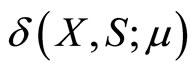 is smaller than a threshold value
  which is obviously true at the start of the first iteration. The following system is used to define the step
 (7)
(7)
where  and
and .
.
Inspired by [8], we used in the third equation for the above system, a linearization , which means that we target the
  -center of
  and
and .
.
After the feasibility step, the new iterates are given by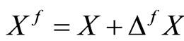 ,
,  and
and . The algorithm begins with an infeasible interior point
  such that
  is feasible for the perturbed problems,
  and
and . First we find a new point
  which is feasible for the perturbed problems with
 . Then
  is decreased to
 . A few centering steps are applied to produce new points
  such that
 . This process is repeated until the algorithm terminates. Starting at the iterates
  and targeting the
  -center, the centering steps are obtained by solving the system (1).
2.3. Infeasible IPMs Based on a Specific Kernel Function
Now we introduce the definition of a kernel function. We call 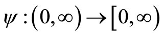 a kernel function if
  is twice differentiable and the following conditions are satisfied
1) 
2)  for all
3) .
.
We define
 (8)
(8)
By using the scaled search directions  and
and  as defined in (4), the system (7) can be reduced to
 (9)
(9)
According to (8), Equation (9) can be rewritten as
 (10)
(10)
It is clear that the right-hand side of the above equation is the negative gradient direction of the following barrier function  whose kernel logarithmic barrier function is
 .
.
Therefore, the aforementioned equation can be rewritten as

Inspired by the work of [4,7,9], and by making a slight modification of the standard Newton direction, the new feasibility step used in this paper, is defined by the following different system:
 (11)
(11)
where the kernel function of  is given by
 (12)
(12)
Since , the third equation in the system (11) can be rewritten as
 (13)
(13)
In the sequel, the feasibility step will be based on the Equation (13).
3. Some Technical Results
We recall some interesting results from Klerk [1]. In the sequel, we denote the iterates after a centrality step as ,
,  ,
, .
.
Lemma 2 Let X, S satisfy the Slater’s regularity condition and . If
. If , then the fullNT step is strictly feasible.
Corollary 3 Let X, S satisfy the Slater’s regularity condition and . If
. If . One has
 .
.
Lemma 4 After a feasible full-NT step the proximity function satisfies
Lemma 5 If , then

The required number of centrality steps can easily be computed. After the  -update, one has
  , and hence after k centrality steps the iterates
  satisfy

From this, one deduces easily that  holds, after at most
 (14)
(14)
We give below a more formal description of the algorithm in Figure 1.
The following lemma stated without proof, will be useful for our analysis.
Lemma 6 (See [10], Lemma 2.5) For any , one has

By applying Lemma (6), one can easily verify so that
for any , we have:
 (15)
(15)
and furthermore, according to (6), we obtain:
 (16)
(16)
Lemma 7 According to the result of Corollary (3), for any  one has

Proof. By applying Hölder inequality and using , we obtain

and the result follows.
The following Lemma gives an upper bound for the proximity-measure of the matrix .
.
Lemma 8 Let  be a primal-dual NT pair and
  such that
 . Moreover let
  and
and . Then

Proof. Since the  is a primal-dual pair and by applying Lemma (7), and the two inequalities (15) and (16), we can get:

since the last term in the last equality is negative. This completes the proof of the Lemma.
Lemma 9 (See [1], Lemma 6.1). If one has  ,
,  , then
 , and
, and .
.
Let Q be an  real symmetric matrix and M be an
  real skew-symmetric matrix, we recall the following result.
Lemma 10 (See [7], Lemma 3.8). If Q is positive definite, then .
.
Lemma 11 (See [1], Lemma 6.3). If Q is positive definite, then .
.
Lemma 12 (See [7], Lemma 3.10). Let A,  ,
,  and
and . Then

Lemma 13 (See [11], Lemma A.1) For , let
, let  denote a convex functions. Then, for any nonzero
 , the following inequality

holds.
4. Analysis of the Feasibility Step
4.1. The Feasibility Step
As established in Section 2, the feasibility step generates new iterates ,
,  and
and  that satisfy the Feasibility conditions for
  and
and  (i.e., primal feasible and dual feasible), except possibly the positive semidefinite conditions. A crucial element in the analysis is to show that after the feasibility step, the inequality
  holds, i.e., that the new iterates are within the region where the Newton process targeting at the
  -centers of
  and
and  is quadratically convergent. Let X, y and S denote the iterates at the start of an iteration and assume that
 . Recall that at the start of the first iteration this is true since
 . Defining
  and
and  as in (4) and
  as in (3). We may write

Therefore  which implies that
 (17)
(17)
According to (8), Equation (13) can be rewritten as
 (18)
(18)
and by multiplying both side from the left with V, we get
 (19)
(19)
To simplify the notation in the sequel, we denote
 (20)
(20)
Note that  is symmetric and M is skew-symmetric. Now we may write, using (19),

By subtracting and adding , to the last expression we obtain

Using (20) and (17), we get
 (21)
(21)
Note that due to (8),  is positive definite.
Lemma 14 Let  and
and . Then the iterates
  are strictly feasible if
 .
.
Proof. We begin by introducing a step length , and we define

We then have ,
,  and similar relations for y and S. It is clear that
 . We want to show that the determinant of
  remains positive for all
 . We may write

By subtracting and adding  and
and
 to the right hand side of the above equality we obtain

where the matrix

is skew-symmetric for all . Lemma (11) implies that the determinant of
  will be positive if the symmetric matrix
is positive definite which is true for all . This means that
  has positive determinant. By positiveness of
  and
and  and continuity of both
  and
and , we deduce that
  and
and  are positive definite which completes the proof.
We continue this section by recalling the following Lemma.
Lemma 15 (See [12], Lemma II. 60). Let  be as given by (6) and
 . Then

The proof of Lemma (15), together with , makes clear that the elements of the vector
  satisfy
 (22)
(22)
Furthermore, by using (8) and (22), we obtain the bounds of the elements of the vector 
 (23)
(23)
In the sequel we denote

where

This implies

and

Lemma 16 Assuming , one has

Proof. Using (6), we get

where 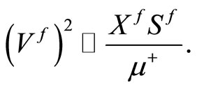
From (21), one has

Due to the fact that  since M is skewsymmetric and Lemma (10), we may write

where we apply for the third equality, Lemma (12) whose second condition is due to the requirement (24) given below.
For each , we define
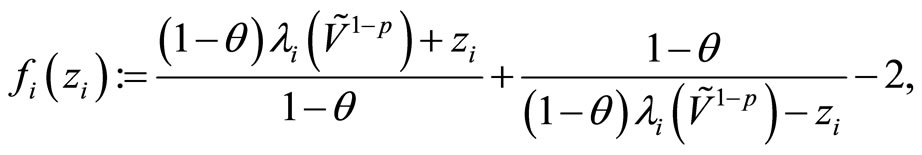
It is clear that  is convex in
  if
if
 . Taking
 , we require

By applying Lemma (15), the above inequality holds if
 (24)
(24)
By using Lemma (13), we may write
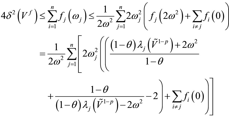
where

Furthermore, by using Lemma (8), we get

We deduce

where

Hence

The last equality is due to (24), which completes the proof.
Because we need to have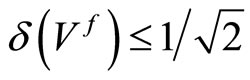 , it follows from this lemma that it suffices if
 (25)
(25)
Now we decide to choose
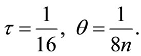 (26)
(26)
Note that the left-hand side of (25) is monotonically increasing with respect to . By some elementary calculations, for
  and
and , we obtain
 (27)
(27)
4.2. Upper Bound for 
In this section we consider the linear space
 .
.
It is clear that the affine space
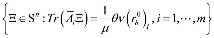
equals  and
and . We can get from Mansouri and Roos [6], the following result.
Lemma 17 (See [6], Lemma 5.11) Let Q be the (unique) matrix in the intersection of the affine spaces  and
and . Then
Note that (27) implies that we must have  to guarantee
 . Due to the above lemma, this will certainly hold if
  satisfies
 (28)
(28)
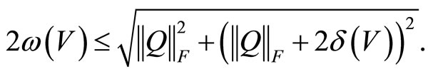
Furthermore, according to Mansouri and Ross, we have

Since , we may write

By using , the above inequality becomes
 (29)
(29)
Because we are looking for the value that we do not allow  to exceed and in order to guarantee that
  , (28) holds if
  satisfies
 , since
 . This will be certainly satisfied if
 . Hence, combining this with (29), we deduce that
  holds.
4.3. Iteration Bound
In the previous sections, we have found that, if at the start of an iteration the iterates satisfies , with
 , then after the feasibility step, with
  as defined in (26), the iterates satisfies
 . According to (14), at most
  centering steps suffice to get iterates that satisfy
 . So each main iteration consists of at most 3 so-called inner iterations. In each main iteration both the duality gap and the norms of the residual vectors are reduced by the factor
 . Hence, using
 , the total number of main iterations is bounded above by

Since , the total number of inner iterations is so bounded above by

5. Concluding Remarks
In this paper we extended the full-Newton step infeasible interior-point algorithm to SDP. We used a specific kernel function to induce the feasibility step and we analyzed the algorithm based on this kernel function. The iteration bound coincides with the currently best known bound for IIPMs. Future research might focuses on studying new kernel functions.
6. Acknowledgements
The authors gratefully acknowledge the help of the guest editor and anonymous referees in improving the readability of the paper.