Differential Evolution Using Opposite Point for Global Numerical Optimization ()
1. Introduction
Global numerical optimization problems arise in almost every field such as industry and engineering design, applied and social science, and statistics and business, etc. The aim of global numerical optimization is to find global optima of a generic objective function. In this paper, we are most interested in the following global numerical minimization problem [1,2]:
 (1)
(1)
where  is the objective function to be minimized,
  is the real-parameter variable vector,
  is the lower bound of the variables and
  is the upper bound of the variables, respectively, such that
 .
.
Many real-world global numerical optimization problems have many objective functions that are non-differentiable, non-continuous, non-linear, noisy, flat, random, or that have many local minima, multiple dimensions, etc. However, the major challenge of the global numerical optimization is that the problems to be optimized have many local optima and multiple dimensions. Such problems are extremely difficult to be optimized and find reliable global optima [3,4]. Therefore, increasing requirements for solving global numerical optimization in various application domains have encouraged many researchers to find a reliable global numerical optimization algorithm. However, in the last decades, this problem remains intractable, theoretically at least [5].
In the global numerical optimization, the traditional methods can be usually classified into two main categories [5,6]: deterministic and probabilistic global numerical optimization methods. During the global numerical optimization process, the first stage is usually to find specific heuristic information involved in problem. Most of deterministic methods rely on the heuristic information to escape from local minima. On the other hand, almost probabilistic methods rely on a probability to determine whether or not search should depart from the neighborhood of a local minimum. Evolutionary algorithms (including genetic algorithm (GA) [7], evolution strategy (ES) [8], genetic programming (GP) [9], and evolutionary programming (EP) [10]) are inspired from the evolution of nature and relatively recent optimization methods. These algorithms have the potential to overcome the limitations of traditional global numerical optimization methods, mainly in terms of unknown system parameters, multiple local minima, non-differentiability, or multiple dimensions, etc. [5,11].
Lately, some new methods for global numerical optimization were gradually introduced. Particle Swarm Optimization (PSO) was originally proposed by J. Kennedy as a simulation of social behavior, and it was initially introduced as an optimization method in 1995 [12]. PSO has been a member of the wide category of Swarm Intelligence methods for solving global numerical optimization problems [13-15]. Differential Evolution (DE) was introduced by Storn and Price in 1995, and developed to optimize real-parameter functions [3,16,17]. DE mainly uses the distance and direction information from the current population to guide its further search, and it mainly has three advantages: 1) finding the true global minimum regardless of the initial parameter values; 2) fast convergence; 3) using a few control parameters. In addition, DE is simple, fast, easy to use, very easily adaptable and useful for optimizing multimodal search spaces [18-22]. Recently, DE has been shown to produce superior performance, and perform better than GA and PSO over some global numerical optimization problems [13,14]. Therefore, DE is very promising in solving global numerical optimization problems.
This paper proposes an opposition-based DE algorithm for global numerical optimization (GNO2DE). This algorithm employs the opposite point method to utilize the existing search spaces to speed the convergence [21-24]. Usually, different problems require different settings for the control parameters. Generally, adaptation is introduced into an evolutionary algorithm, which can improve the ability to solve a general class of problems, without user interaction. In order to improve the adaptation and reduce the control parameter, GNO2DE uses a dynamic mechanism to dynamically tune the crossover rate CR during the evolutionary process. Moreover, GNO2DE can enhance the search ability by randomly selecting a candidate from strategies “DE/rand/1/bin” and “DE/current to best/2/bin”. Numerical experiments clearly show that GNO2DE is feasible and effective.
The remainder of this paper is organized as follows. Section 2 briefly introduces the basic idea of the DE algorithm. Section 3 describes in detail the proposed GNO2DE algorithm. Section 4 presents the experimental setup adopted and provides an analysis of the experimental results obtained from our empirical study. Finally, our conclusions and some possible paths for the future research are provided in Section 5.
2. The Classical DE Algorithm
The DE algorithm is a population-based stochastic optimization algorithm like many evolutionary algorithms such as genetic algorithms using three similar genetic operators: crossover, mutation, and selection [7]. The main difference in generating better solutions is that genetic algorithms mainly rely on crossover while DE mainly relies on mutation operation. The DE algorithm uses mutation operation as a search mechanism and selection operation to direct the search toward the prospective regions in the search space. The DE algorithm also uses a non-uniform crossover that can take child vector parameters from one parent more often than it does from others. By using the components of the existing population members to generate trial vectors, the recombination (i.e., crossover) operator efficiently shuffles information about successful combinations, enabling the search for a better solution space [3,16,17].
A global numerical optimization problem consisting of n parameters can be represented by a n-dimensional vector. In DE, a population of  solution vectors is randomly created at the start, where
 . The population is successfully improved by applying mutation, crossover, and selection operators [13,25,26].
2.1. Randomly Initializing Population
Like other many evolutionary algorithms, the DE algorithm starts with an initial population, which is randomly generated when no preliminary knowledge about the solution is available. In DE, let us assume that an individual  stands for the
  individual of population
  (population size
 ) at the generation
 . The population
  is initialized as
 (2)
(2)
where  is the population size,
  is the number of variables,
  is a uniformly distributed random number in the range [0,1], and
  is the
  variable of the
  individual at the initial generation, which is initialized within the
  range
range .
.
2.2. Mutation Operation
In the mutation phase, DE randomly selects three distinct individuals from the current population. For each target vector , the
, the  mutant vector is generated based on the three selected individuals as follows:
 (3)
(3)
where , random indexes
  are randomly chosen integers, mutually different, and they are also chosen to be different from the running index
 , so that
  must be greater or equal to four to allow for this condition. The scaling factor
  is a control parameter of the DE algorithm, which controls the amplification of the differential variation (
 ). And the scaling factor
  is a real constant factor in the range
  and is often set to 0.5 in the real applications [27].
The above strategy is called “DE/rand/1/bin”, it is not the only variant of DE mutation which has been proven to be useful for real-valued optimization. In order to classify the variants of DE mutation, the notation:  is introduced where 1)
  specifies the vector to be mutated which currently can be “rand” (a randomly chosen population vector) or “best” (the vector of lowest cost from the current population); 2)
  is the number of difference vectors used; 3)
  denotes the crossover scheme, there are two crossover schemes often used, namely, “bin” (i.e., the binomial recombination) and “exp” (i.e., the exponential recombination). Usually, there are the following several differential DE schemes often used in the global optimization [3]:
“DE/best/1/bin”:
 (4)
(4)
“DE/current to best/2/bin”:
 (5)
(5)
“DE/best/2/bin”:
 (6)
(6)
“DE/rand/2/bin”:
 (7)
(7)
where  is the best individual of the current population
 . The scaling factor
  is the control parameter of the DE algorithm.
2.3. Crossover Operation
In order to increase the diversity of the perturbed parameter vectors, the crossover operator is introduced. The new individual is generated by recombining the original vector  and the mutant vector
  according to the following formula:
 (8)
(8)
where  stands for a uniformly distributed random number in the range [0,1], and
  is a randomly chosen index from the set
  to ensure that at least one of the variables should be changed and
  does not directly duplicate
 . And the crossover rate
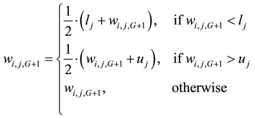
  is a real constant in the range [0,1], one of control parameters of the DE algorithm. After crossover, if one or more of the variables in the new solution are outside their boundaries, the following repair rule is applied [25]:
 (9)
(9)
2.4. Selection Operation
After mutation and crossover, the selection operation selects to decide that the new individual  or the original individual
  will survive to be a member of the next generation. If the fitness value of the new individual
  is better than that of the original one
  then the new individual
  is to be an offspring in the next generation (G + 1) else the new individual
  is discarded and the original one
  is retained in the next generation. For a minimization problem, we can use the following selection rule:
 (10)
(10)
where  is the fitness function, and
  is the offspring of
  in the next generation (G + 1).
2.5. The General Framework of the DE Algorithm
The above operations (i.e., mutation, crossover, and selection) are repeated  (population size) times to generate the next population of the current population. These successive generations are generated until the predefined termination criterion is satisfied. The main steps of the DE algorithm are given in Figure 1.

Figure 1. The generic framework of the DE algorithm.
3. The Proposed GNO2DE Algorithm
Similar to all population-based optimization algorithms, two main steps are distinguishable for the DE, population initialization and producing new generations by evolutionary operations such as selection, crossover, and mutation. GNO2DE enhances these two steps using the opposite point method. The opposite point method has been proven to be an effective method to evolutionary algorithms for solving global numerical problems. When evaluating a point to a given problem, simultaneously computing its opposite point can provide another chance for finding a point closer to the global optimum. The concept of the opposite point is defined as follows [21- 24]:
Definition 1 Let us assume that  is the
  point of the population
  (population size
 ) at the generation
  in the n-dimensional space. The opposite point
 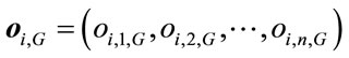 is completely defined by its components as follows:
 (11)
(11)
where ,
,  ,
,  and
and  are the lower and the upper limits of the variable
 , respectively.
3.1. Generating the Initial Population Using the Opposite Point Method
Generally, population-based Evolutionary Algorithms randomly generate the initial population within the boundaries of parameter variables. In order to improve the quality of the initial population, we can obtain fitter starting candidate solutions by utilizing opposite points, even when there is no a priori knowledge about the solution (s). The procedure of generating the initial population using the opposite point method is given as follows:
Step 1: Randomly initialize the starting population  (population size
 ).
).
Step 2: Calculate the opposite population of  using the opposite point method, and obtain the opposite population
 .
.
Step 3: Select the fittest individuals from
  as the initial population
 .
.
3.2. Evolving the Population Using the Opposite Point Method
By applying a similar approach to the current population, the evolutionary process can be forced to jump to a new solution candidate, which may be fitter than the current one. After generating new population by selection, crossover, and mutation, the opposite population is calculated and the  fittest individuals are selected from the union of the current population and the opposite population. Following steps describe the procedure:
Step 1: The offspring population  of the current population
  is generated after performing the corresponding successive DE operations (i.e., mutation, crossover, and selection).
Step 2: Calculate the opposite population of  using the opposite point method, and obtain the opposite population
 .
.
Step 3: Select the  fittest individuals from
  as the next generation population
 .
.
Step 4: Let .
.
3.3. Adaptive Crossover Rate CR
In DE, the aim of crossover is to improve the diversity of the population, and there is a control parameter  (i.e., the crossover rate) to control the diversity. The smaller diversity is easy to result in the premature convergence, while the larger diversity reduces the convergence speed. In conventional DE, the crossover rate
  is a constant value in the range [0,1]. Inspired by nonuniform mutation, this paper introduces an adaptive crossover rate
 , which is defined as follows [28]:
 (12)
(12)
where  is a uniform random number from [0,1],
  and
and  are the current generation number and the maximal generation number, respectively. The parameter
  is a shape parameter determining the degree of dependency on the iteration number and usually is set to 2 or 3. In this study,
  is set to 3.
The property of  causes the crossover operator to search the solution space uniformly initially when
  is small, while to search the solution space very locally when
  is large. This strategy increases the probability of generating a new number close to its successor than a random choice. Therefore, at the early stage, GNO2DE uses a bigger crossover rate
  to search the solution space to preserve the diversity of solutions and prevent premature convergence; at the later stage, GNO2DE employs a smaller crossover rate
  to search the solution space to enhance the local search and prevent the fitter solutions found from being destroyed. The relation of generation vs crossover rate
  is plotted in Figure 2.
3.4. Adaptive Mutation Strategies
In subsection 2.2, we have described a few useful mutation schemes, where “DE/rand/1/bin” and “DE/current to best/2/bin” are the most often used in practical applications mainly due to their good performance [17,19]. To overcome their respective disadvantages and utilize their

Figure 2. The graph for generation vs crossover rate CR.
cooperative advantages, GNO2DE randomly chooses a mutation scheme from two candidates “DE/rand/1/bin” (i.e., Equation (3)) and “DE/current to best/2/bin” (i.e., Equation (5)), and the new mutant vector  is generated according to the following formula [27]:
 (13)
(13)
where  is a uniform random number from the range [0,1].
3.5. Approaching of Boundaries
In the given optimization problem, it has to be ensured that some boundary values are not outside their limits. Several possibilities exist for this task: 1) The positions that beyond the boundaries are newly generated until the positions within the boundaries are satisfied; 2) the boundary-exceeding values are replaced by random numbers in the feasible region; 3) The boundary is approached asymptotically by setting the boundary-offending value to the middle between old position and boundary [29]:
 (14)
(14)
After crossover, if one or more of the variables in the new vector  are outside their boundaries, the violated variable value
  is either reflected back from the violated boundary or set to the corresponding boundary value using the repair rule as follows [30]:
 (15)
(15)
where  is a probability and a uniformly distributed random number in the range [0,1].
3.6. The Framework of the GNO2DE Algorithm
DE creates new candidate solutions by combining the parent individual and several other individuals of the same population. A candidate replaces the parent only if it has better fitness value. The initial population is selected randomly in a uniform manner between the lower and upper bounds defined for each variable. These bounds are specified by the user according to the nature of the problem. After initialization, DE performs mutation, crossover, selection etc., in an evolution process. The general framework of the GNO2DE algorithm is described in Figure 3.
4. Numerical Experiments
4.1. Benchmark Functions
In order to test the robustness and effectiveness of GNO2DE, we use a well-known test set of 23 benchmark functions [1,2,31-33]. This relatively large set is necessary in order to reduce biases in evaluating algorithms.

Figure 3. The general framework of GNO2DE.
The complete description of all these functions and the corresponding parameters involved are described in Table 1 and APPENDX. These functions can be divided into three different categories with different complexities:

Table 1. The 23 benchmark test functions .
.
1) unimodal functions ( ), which are relatively easy to be optimized, but the difficulty increases as the dimensions of the problems increase (see Figure 4); 2) multimodal functions (
 ), which have many local minima, represent the most difficult class of problems for many optimization algorithms (see Figure 5); 3) multimodal functions (
 ), which contain only few local optima (see Figure 6). It is interesting to note that some functions have unique features:
  is a discontinuous step function having a single optimum;
  is a noisy function involving a uniformly distributed random variable within the range [0,1]. In unimodal functions the convergence rate is our main interest, as the optimization is not a hard problem. Obviously, for multimodal functions the quality of the final results is more important because it reflects the ability of the designed algorithm to escape from local optima.
4.2. Discussion of Parameter Settings
In order to setup the parameters, we firstly discuss the convergence characteristic of each function of dimen-

Figure 4. Graph for one unimodal function.

Figure 5. Graph for one multimodal function with many local minima.

Figure 6. Graph for one multimodal function containing only few local optima.
sionality 30 or lower. The parameters used by GNO2DE are listed in the following: the control parameter , the population size
 , the maximal generation number
  for functions
 ,
,  ,
,  for functions
 , respectively. For convenience of illustration, we plot the convergence graphs for benchmark test functions
  in Figures 7-12.
Figures 7-12 clearly show that GNO2DE can achieve better convergence for each function of ,
,  ,
,  , and
, and , when evaluated by 100,000 FES (the number of fitness evaluations). From Figure 8, we know that function
  approximately requires 300,000 FES to achieve the convergence, and that the convergence speed of function
  is relatively slow in the case of the above parameters. Therefore, in order to investigate the effect of the control parameter
  on the convergence. Some experimental results are given in Figures 13-18. Firstly, the control parameter
  is set to different values 0.4, 0.5, 0.6, 0.7 on functions
  and
and , and the convergence curve is presented in Figures 13 and 14. From Figures 13 and 14, we can observe that GNO2DE can achieve the convergence for each value of the above control parameter F when the number of fitness evaluations is set to 100,000 FES, while the convergence speed is fastest when the value of the control parameter
  is set to 0.5. For function
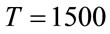
 , we set the control parameter
  to 0.5, 0.6, 0.7, and 0.8, respectively. The convergence graph is given in Figure 15. From Figure 15, it is clearly shown that the convergence speed is obviously fastest when the value of the control parameter
  is set to 0.6. In addition, we also present the convergence graph of each function of
 ,
,  , and
, and  in Figures 16-18, respectively. The control parameter
  is set to 0.5, 0.6, 0.7, and 0.8. From these figures, we can institutively find that the convergence speed is relatively fastest when the value of the control parameter is set to 0.5.

Figure 7. Convergence graph for functions .
.

Figure 8. Convergence graph for functions .
.

Figure 9. Convergence graph for functions .
.

Figure 10. Convergence graph for functions .
.

Figure 11. Convergence graph for functions .
.

Figure 12. Convergence graph for functions .
.

Figure 13. Convergence curve of  for each F value.

Figure 14. Convergence curve of  for each F value.

Figure 15. Convergence curve of  for each F value.
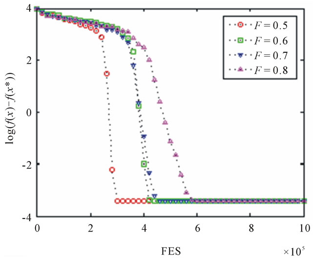
Figure 16. Convergence curve of  for each F value.

Figure 17. Convergence curve of  for each F value.

Figure 18. Convergence curve of  for each F value.
Therefore, for the most functions, GNO2DE can show good performance when the value of the control parameter  is set to 0.5 or 0.6. According to the above discussion and analysis, we set up the corresponding experimental parameters in Tables 2-4. Table 2 presents the parameters used by GNO2DE, GNO2DE-A, and GNO2DE-B for functions of dimensionality 30 or lower, where GNO2DE-A and GNO2DE-B employ only DE schemes “DE/rand/1/bin” or “DE/current to best/2/bin”, respectively. Table 3 presents the parameters used by GNODE (without using the opposite point method) for functions of dimensionality 30 or lower. Table 4 presents the parameter settings used by GNO2DE for functions of dimensionality 100.
4.3. Comparison of GNO2DE with GNODE
In this section, we compare GNO2DE with GNODE in terms of some performance indices according to the parameter settings presented in Tables 2 and 3. The experimental results are in detail summarized in Tables 5 and 6, and better results are highlighted in boldface. The optimized objective function values over 30 independent runs are arranged in ascending order and the 15th value in the list is called the median optimized function value.
According to Tables 5 and 6, we can find that GNO2DE

Table 2. Parameters used by GNO2DE, GNO2DE-A, and GNO2DE-B for functions of dimensionality 30 or lower.

Table 3. Parameters used by GNODE for functions of dimensionality 30 or lower.

Table 4. Parameters used by GNO2DE for functions of dimensionality 100.
can obtain the optima or near optima with certain precision for all test functions  of dimensionality 30 or less. For each function of
 ,
,  ,
,  ,
,  ,
,  ,
,  ,
,  , and
, and , the performance of GNO2DE is superior to or less worse than the performance of GNODE in terms of the min value (i.e., the best result), the median value (i.e., the median result), the max value (i.e., the worst result), the mean value (i.e., the mean result), and the std value (i.e., the standard deviation result), on condition that while the FES of GNO2DE is essentially less than that of GNODE, although they are apparently set to the same FES 100,000. In addition, the global optimum of function
  found by GNO2DE is f18(x) = 2.99999999999992, the corresponding x = (0.00000000061668, −0.99999999932877).
According to Table 5, for , the performance of GNO2DE is obviously better than that of GNODE in terms of the max, mean, and std values, while the performance of GNODE is slightly better than that of GNO2DE in terms of the min, median values. For
 , the median, max, mean, and std values of GNODE are better than those of GNO2DE, while the min value of GNODE is approximate to that of GNO2DE. For
 , the min, median, max, and mean values of GNO2DE are better than those of GNODE, while the std value of GNO2DE is worse than that of GNODE. The reason is that GNO2DE can’t find the optimal solution in very few runs of 30 runs. For function
 , the min, median, max, mean, and std values of GNO2DE are slightly worse than those of GNODE.
As shown in Table 6, for , the min, median values of GNO2DE are similar to those of GNODE, while the max, mean, and std values of GNO2DE are worse than those of GNODE to some extent. This is because that GNO2DE can’t obtain the min value in one or two runs of 30 runs. For
 , the min, and max values obtained by GNO2DE are the same to those by GNODE, while the median value obtained by GNO2DE is worse than that obtained by GNODE. Accordingly, it also decides that the mean, and std values of GNO2DE are worse than those of GNODE. GNO2DE and GNODE all have a tendency to getting stuck in the local optima. The global optima of function
  found by GNO2DE is f20(x) = −3.33539215295525, the corresponding x = (0.20085810809731, 0.15013171771783, 0.47865329178970, 0.27652528463205, 0.31191293322300, 0.65702016661775).
In conclusion, the performance of GNO2DE is relatively stable and obviously better than or not worse than that of GNODE. The reason is that GNO2DE uses the opposite point method to provide another chance for finding a solution more close to the global numerical optimum, without increasing much time.

Table 5. Comparison between GNO2DE, and GNODE on functions  of dimensionality 30.
4.4. Comparison of GNO2DE with GNO2DE-A, and GNO2DE-B
In this section, we compare GNO2DE (“DE/rand/1/bin” and “DE/current to best/2/bin”) with GNO2DE-A (“DE/ rand/1/bin”), and GNO2DE-B (“DE/current to best/2/ bin”) in terms of the best result (i.e., the min value), the mean result (i.e., the mean value), and the standard deviation result (i.e., the std value). The parameter settings of GNO2DE, GNO2DE-A, and GNO2DE-B are given in
Table 2. The experimental results are in detail summarized in Tables 7 and 8, and better results are highlighted in boldface. The optimized objective function values over 30 independent runs are arranged in ascending order and the 15th value in the list is called the median optimized function value.
From Tables 7 and 8, it is clearly shown that for each function of ,
,  ,
,  ,
,  , the min, mean, and std values of GNO2DE are similar to those of

Table 6. Comparison between GNO2DE, and GNODE on functions .
.
GNO2DE-A, and GNO2DE-B, and three algorithms all can find the optimal solution.
Table 7 shows that for each function of , the optimal solution can be found by GNO2DE, GNO2DE-A, and GNO2DE-B, while the mean, std values of GNO2DE are slightly different from those of GNO2DE-A, and GNO2DE-B. For
 , the mean, and std values of GNO2DE are obviously better than those of GNO2DE-A, and GNO2DE-B, while the min value of GNO2DE-A is worst among three algorithms. For
 , the min value of GNO2DE-A is best among three algorithms, while its mean, and std values are worse or not better than those of GNO2DE, and GNO2DE-B. For
 , the min, mean, and std values of GNO2DE-B are obviously worse than those of GNO2DE, and GNO2DE-A, while GNO2DE-A can obtained better mean, and std values than GNO2DE. For
 , the min value of GNO2DE-A is worst among three algorithms, while the std value of GNO2DE is best among three algorithms. For
 , the min value of GNO2DE-A is worst among three algorithms, while the mean, and std values of GNO2DE are best among three algorithms.
Table 8 shows that for , the min, and mean values are approximate among three algorithms, while the std value of GNO2DE is best, that of GNO2DE-B is better, and that of GNO2DE-A is good. For
 , the min, and mean values are similar among three algorithms, while the std value of GNO2DE-B is best, that of GNO2DE is better, and that of GNO2DE-A is good.
Therefore, from the above analysis, we know that the performance of GNO2DE is more stable than that of GNO2DE-A, and that of GNO2DE-B. This is because that GNO2DE employs two schemes “DE/bin/1/bin” and “DE/current to best/2/bin” to search the solution space. On the whole, GNO2DE can improve the search ability.
4.5. Comparison of GNO2DE with Some State-of-the-Art Algorithms
In this section, we compare GNO2DE with DE [3], ODE/2 [2], SOA [31], FEP [32], opt-IA [1], and CLPSO [15] in terms of the mean result (i.e., the mean value), the standard deviation result (i.e., the std value), and the

Table 7. Comparison between GNO2DE, GNO2DE-A, and GNO2DE-B on functions  of dimensionality 30.

Table 8. Comparison between GNO2DE, GNO2DE-A, and GNO2DE-B on functions .
.
number of fitness evaluations (i.e., the FES value). The statistical results are summarized in Tables 9 and 10, and better results are highlighted in boldface. The experimental results of DE, SOA, and CLPSO are taken from [31], and the experimental results of ODE/2, FEP are taken from [2]. The optimized objective function values of 30 runs are arranged in ascending order and the 15th value in the list is called the median optimized function value. Table 9 clearly shows that the mean, std values of GNO2DE are obviously superior to those of DE, ODE/2, SOA, FEP, opt-IA, and CLPSO on ,
,  ,
,  , while GNO2DE uses the least FES 100,000 among these methods, that the mean, std values of SOA are slightly better than those of GNO2DE, ODE/2, DE, etc. on
 ,
,
Table 9. Comparison between GNO2DE, DE, ODE/2, SOA, FEP, opt-IA, and CLPSO on functions  of dimensionality 30.

Table 10. Comparison between GNO2DE, DE, ODE/2, SOA, FEP, opt-IA, and CLPSO on functions .
.
 ,
,  , while the 100,000 FES of GNO2DE is least among these methods, and that the mean, std, FES values of GNO2DE are better than DE, ODE/2, FEP, opt-IA, and CLPSO. For
 ,
,  ,
,  , the mean, std, and FES values of ODE/2 are not worse than or better than those of other methods. For
 , compared with DE, GNO2DE is slightly worse in terms of the mean, std values of, while the 200,000 FES of DE is twice of that of GNO2DE, and the performance of GNO2DE is clearly better than that of SOA, FEP, opt-IA, and CLPSO. For
 , the mean, std values of GNO2DE are similar to those of DE, SOA, FEP, opt-IA, and CLPSO, while the 100,000 FES used by GNO2DE is least among these methods. For
 , the mean, std, FES values of GNO2DE are obviously better than those of DE, SOA, FEP, opt-IA, and CLPSO. For
 ,
,  , the min, std values of ODE/2 are better than those of other methods, while the 100,000 FES used by GNO2DE is least among these methods.
As shown in Table 10, the mean value of GNO2DE and SOA on  is approximate and are better than other methods, while ODE/2 has the least std, and FES values. For
 , all methods have the similar performance. For
 , GNO2DE, DE, ODE/2, SOA, CLPSO have the similar performance and are better than FEP. For
 , the performance of ODE/2 and FEP is better than other methods. For
 , the performance of GNO2DE, DE, and ODE/2 is approximate and are better than other methods.
In sum, the mean and standard deviation results of GNO2DE are not worse than or superior to DE, ODE/2, SOA, FEP, opt-IA, and CLPSO on a test set of benchmark functions. GNO2DE uses the opposite point method, employs two DE schemes “DE/rand/1/bin” and “DE/ current to best/2/bin”, and introduces non-uniform crossover rate. These techniques are beneficial to enhancing the performance of GNO2DE.
4.6. Experimental Results of 100-Dimensional Functions
In this section, the statistical results of GNO2DE on 100- dimensional functions are given in Table 11. The parameter setup is used in Table 4. The optimized objecttive function values over 30 independent runs are arranged in ascending order and the 15th value in the list is called the median optimized function value. Table 11 clearly shows that GNO2DE can find the optimum or near optimum of each 100-dimensional function of , and that GNO2DE can obtain the stable performance of each function of
 ,
,  , while it performs slightly worse on
 ,
,  ,
, . Therefore, when used for solving high dimensional global numerical optimization problems, NGO2DE also performs well.
5. Conclusion and Future Work
This paper introduces an opposition-based DE algorithm for global numerical optimization (GNO2DE). GNO2DE uses the method of opposition-based learning to utilize the existing search spaces to improve the convergence speed, employs adaptive DE schemes and non-uniform crossover to enhance the adaptive search ability. Numerical results show that GNO2DE outperforms some stateof-the-art algorithms. However, there are still some possible things to do in the future: 1) further, to improve the self-adaptation of the control parameters such as the scaling factor F; 2) to test higher dimensional global nu-

Table 11. Experimental Results of 100-dimensional functions .
.
merical optimization problems; 3) to introduce some local search and heuristic techniques to speed up the convergence and escape from the local optima, etc.
Appendix
 ,
, 
 ,
, 


