1. Introduction
The particle decays in the Standard Model are characterized by their decay width Γ (or equivalently decay rate
), and are described by the famous Fermi’s golden rule, i.e. an integral with parameters.
A closed expression for Γ can be found in only a few cases, otherwise there are empirical formulas, or simply data tables.
We present here a two-step calculation method for calculation of general decay rates in the Standard Model.
The first step is a phenomenological classification method, which is an improved and generalized schematic formula for decay width originally introduced by Chang [1] . It is a general parameterized approximation formula with some special cases, which is in good agreement with measurements.
It introduces seven classes of particle decays, where the interaction constant is roughly class-specific. In other words, it allows to extrapolate and make assessments for decays, for which there is no analytic formula. Furthermore, it supports the notion of decay-mediating virtual particle with interaction energy mX.
The second step is a numerical Lagrangian calculation method for interaction energy mX, which calculates the interaction energy of the process numerically by minimization of action from the Lagrangian of the process. From the interaction energy follows the decay width using the phenomenological formula. A comparison of numerically calculated and observed decay widths for a large selection of decays shows a good agreement.
The starting point for decay rate
, or equivalently, its decay width Γ, of a n-body process
is the Fermi’s golden rule
We demonstrate in chap.2 at selected examples, how to derive Γ from Fermi’s golden rule in a closed form, which in general has to be done numerically.
For 2-body decays and 3-body decays we can (approximately) split-off the kinematic factor
of Γ, taking the transition matrix out of the integral.
The phenomenological classification method is described in chap.3 and chap. 5, and the calculated
are compared with measured
in chap.6.
The phenomenological formula for the decay width is [1] .
, where
Legendre polynomial m = l or m = l + 1, l = isospin I,
mass ratio,
with G = interaction
constant,
is the initial mass, k is the mass-power-coefficient.
We introduce and derive the interaction energy mX in the form
.
The numerical calculation method is based on an extended version of the Standard Model (SM) introduced by Helm [2] , called the extended SU(4)-preon-model (SU4PM). In SU4PM, the Pauli SU(2)-weak interaction is extended to SU(4)-hypercolor (hc) interaction with four charges, 15 hc-boson fields and two subparticles called preons, and SU(2)-weak interaction becomes a Yukawa-approximation via massive (W, Z)-bosons.
The SU4PM model allows to calculate the masses of the SM remarkably well, reducing 29 parameters of the SM to 7.
In chap. 7, we calculate the interaction energy mX numerically by minimization of action of the SU4PM Lagrangian of the particles in the decay process, and we obtain a good agreement between the calculated values
and observed values
.
A remark about units: in particle physics it is customary to use the convention
, and we adopt it here as well, except in places, where quantities have to be distinguished, e.g. decay width Γ is an energy and is measured in MeV:
, whereas decay rate
is measured in s−1:
.
Other quantities are transformed from each other by
and c, e.g. mass
, time
, length
, angular momentum
.
The contents of the paper is as follows.
In chap. 2, first some important decays are discussed, and in 1.8 and 1.9 the general decay width formula for 3-body and 2-body decays.
In chap. 3 the phenomenological formula for the decays is presented, and is discussed for some important decays.
Chap. 4 shows the data of the most important particles.
In chap. 5, the phenomenological formula values and the observed values for the decay width, together with the decay interaction energy mX are discussed.
In chap. 6 the phenomenological decay width, the observed decay width, and the interaction energy are shown in a table and in a plot, and generally characterized.
In chap. 7, we present a calculation method and a reaction model using electromagnetic, color SU(3), and extended weak SU(4) interaction based on SU4PM model.
Here, the theoretical background and the calculation software is discussed, and the calculated results for
are compared to the observed values
from chap. 5, and shown in a table and in plots.
2. Selected Particle Decays with Theoretical Background
In this chapter we discuss some well-understood particle decays, with decay width described by an analytical formula [3] [4] [5] [6] [7] .
2.1. Neutron
The free neutron decays into a proton, electron, and antineutrino [8] is shown in Figure 1.
The rest energy
is carried away by e and ν
The transition matrix of the decay is [8] [10]
from the interaction Hamiltonian [10]
with
is the Fermi weak coupling constant,
(V is the CKM-matrix),
and the weak V-constant is
,
and λ is the hadronic strong interaction correction.
We compute the neutron decay probability per unit time using Fermi’s golden rule [11] :
, where
= final state energy density
or in differential form [11]
(1)
where
,
,
,
,
with the (dimensionless) transition matrix
of the interaction Hamiltonian
.
Here Ee, pe, En, and pn are the electron and antineutrino total energy and momentum Δ is the neutron-proton mass difference
.
Integration over the antineutrino and electron momenta gives the beta electron energy spectrum
Additional integration over electron energy yields
Here fR is the phase-space term, i.e. the value of the integral over the Fermi energy spectrum, including Coulomb, recoil order, and radiative corrections.
The decay width of the decay becomes [8]
(2)
where
,
,
,
,
with the phase-space term [9]
,
,
here the transition probability per unit time is
.
The neutron lifetime τn becomes
2.2. Muon
The muon decays into an electron, an electron-antineutrino and a muon-neutrino is shown in Figure 2.
For the muon decay we derive the formula for the decay width Γ [6] [12] .
The interaction Hamiltonian is the current-current interaction
From the transition matrix element
with
and G = GF, g is the weak dimensionless interaction constant,
we obtain after some γ-algebra averaging over the spins and trace-manipulation.
and for the decay rate we have Fermi’s golden rule
In the muon rest frame
and
and with
in spherical coordinates
with variable
,
and with E = k4
we obtain
,
(3)
and the decay time
,
where
,
or in seconds, multiplied by
,
we obtain the lifetime
.
2.3. Tauon
The decay modes of the tauon are
The leptonic modes give a factor
, the hadronic modes a factor
,
and
2.4. Pions
The particle data for the pions are shown in Table 1.
Charged pion decays
The diagram of charged pion decays is shown in Figure 3.
The π± mesons have a mass of 139.6 MeV/c2 and a mean lifetime of 2.6033 × 10⁻⁸ s. They decay due to the weak interaction. The primary decay mode of a pion, with a branching fraction of 0.999877, is a leptonic decay into a muon and a muon neutrino:
The pion-muon decay width is [14]
![]()
Figure 3. Feynman diagram of the dominant leptonic pion decay [13] .
where
is the (dimensionless) pion decay factor,
.
The second most common decay mode of a pion, with a branching fraction of 0.000123, is also a leptonic decay into an electron and the corresponding electron antineutrino. This “electronic mode” was discovered at CERN in 1958
The suppression of the electronic decay mode with respect to the muonic one is given approximately (up to a few percent effect of the radiative corrections) by the ratio of the half-widths of the pion-electron and the pion-muon decay reactions:
and is a spin effect known as helicity suppression.
Also observed, for charged pions only, is the very rare “pion beta decay” (with branching fraction of about 10−8) into a neutral pion, an electron and an electron antineutrino (or for positive pions, a neutral pion, a positron, and electron neutrino).
The rate at which pions decay is a prominent quantity in many sub-fields of particle physics, such as chiral perturbation theory. This rate is parametrized by the pion decay constant (ƒπ), related to the wave function overlap of the quark and antiquark, which is about 130 MeV.
Neutral pion decays
The π0 meson has a mass of 135.0 MeV/c2 and a mean lifetime of 8.4 × 10⁻¹⁷ s. It decays via the electromagnetic force, which explains why its mean lifetime is much smaller than that of the charged pion (which can only decay via the weak force).
The neutral pion decay is shown in Figure 4.
The dominant π0 decay mode (anomaly-induced neutral pion decay), with a branching ratio of BR = 0.98823, is into two photons:
![]()
Figure 4. Anomaly-induced neutral pion decay [13] .
The second largest π0 decay mode (BR = 0.01174) is the Dalitz decay (named after Richard Dalitz), which is a two-photon decay with an internal photon conversion resulting a photon and an electron-positron pair in the final state:
The third largest established decay mode (BR = 3.34 × 10⁻⁵) is the double Dalitz decay, with both photons undergoing internal conversion which leads to further suppression of the rate:
The fourth largest established decay mode is the loop-induced and therefore suppressed (and additionally helicity-suppressed) leptonic decay mode (BR = 6.46 × 10⁻⁸):
2.5. Pion-Nucleon Interaction and Decays
The Lagrangian is [6] [15]
with pion
, nucleon
, and Pauli-matrix-vector
, explicitly
with Feynman diagrams shown in Figure 5.
and with the corresponding hadronic transformations
,
,
,
![]()
Figure 5. Nucleon interaction via pions.
2.6. Kaons
Kaons exist in charged form ch-kaon =
and neutral form n-kaon =
, where n-kaon appears in nature as a symmetric and antisymmetric mixture of d and s: the long-lived kaon-L and the short-lived kaon-S.
The particle data for the kaons are shown in Table 2, their decay reactions in Table 3, and their quark decay processes in Figure 6.
![]()
Table 3. Main decay modes for K+ [16] .
![]()
Figure 6. Quark diagrams for K+ and K0 decays involving strangeness changing neutral currents [10] .
K0 decay and CP-violation
The full kaon-L and kaon-S contain a CP-violating term:
CP violation factor.
2.7. The Kaon-Pion Decay Detailed Theory
In [17] a semi-empirical formula for the transition matrix element
in
is derived.
First, the kinematic momentum variables s0, s1, s2, s3 are introduced
,
,
,
then, the Dalitz plot variables
,
are defined.
We obtain for
(x,y) the expression
with the constants:
,
,
,
,
,
,
,
,
and
,
.
We obtain the following expression for the differential transition width from Fermi’s golden rule:
or, with Dalitz variables
we choose
,
, i.e.
,
,
,
,
We insert
and calculate Γ as an integral over
,
θ12, integration
cancels out
and changing to E1, E2, θ12:
,
,
,
we solve dΓ for E2 [2] :
and
now we carry out the integration over E2 with the delta-function:
and after simplification
(4)
The integration boundary in E1 is
, in θ12
where
is the relative momentum, at which E2 becomes
complex
Numerical integration yields for
,
[2] .
, the measured decay width is 0.0297 × 10⁻¹⁶ GeV (see below).
2.8. The General 3-Body Decay
We use the momentum notations
[14] [18] .
We start again with Fermi’s golden rule:
(5)
we choose
,
, i.e.
,
,
,
,
now we calculate Γ as an integral over
,
θ12, integration
cancels out
and changing to E1, E2, θ12:
,
,
,
we solve for E2 [2] :
and
now we carry out the integration over E2 with the delta-function:
and after simplification
setting
we obtain the partial kinematic factor for 3-body
decay
(6)
The integration boundary in E1 is
, in θ12
where
is the relative momentum, at which E2
becomes complex
(6a)
The kinematic factor
can be calculated numerically.
The total kinematic factor results from
by symmetrization over all 6 index permutations
Here is the plot of
shown in Figure 7.
Example:
with kinematic factor:
.
2.9. The General 2-Body Decay
We use the momentum notations
[14] [18] .
We start again with Fermi’s golden rule for 2-body decay [11] :
(7)
we choose
,
, i.e.
,
,
,
![]()
Figure 7. Plot of
.
now we calculate Γ as an integral over
, integration
cancels out
and changing to
:
,
from
we obtain the solution [2]
,
the integration
cancels out and we obtain, setting
(8)
we obtain the kinematic factor for 2-body decay
(8a)
The total kinematic factor for 2-body decay results from the symmetrized
As an example, here is the plot
shown in Figure 8.
Example:
, with kinematic factor:
.
![]()
Figure 8. Plot of
.
3. The Theoretical Background and the Phenomenological Decay Formula
Schematics: decay width phenomenological formula, interaction energy
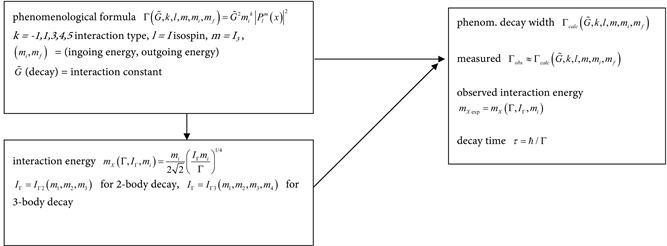
In this chapter, we follow the following scheme underlying the phenomenological formula by Chang [1] for decay width, the derived interaction energy, and resulting decay time.
The phenomenological formula is a semi-empirical scheme for the calculation of the decay width Γ of a decay:
, depending on
= (ingoing energy, outgoing energy), interaction constant (decay dependent)
, interaction type k = −1, 1, 3, 4, 5, and extended isospin I with the traditional notations l = I, m = I3.
From the decay width, the decay time follows immediately
.
The agreement between the phenomenological
and the observed values
is remarkably good (see chap. 6).
The interaction energy
between the incoming and the outgoing state in the process (corresponding to the energy of the mediating particle in the Feynman diagram, e.g.
boson in the neutron decay), can be calculated from Γ using kinematics factors
.
The kinematics factors describe the statistics of the process and depend on the involved particle masses.
In 1.8 and 1.9 we calculated the kinematic factor and obtained for decay width the general formula
.
The formula for interaction energy
is derived
below in chap. 3.1.
3.1. The Phenomenological Decay Formula and Interaction Energy
The phenomenological decay formula
The phenomenological formula for the decay width is [1]
(9)
where
Legendre polynomial
or
, l = isospin I,
mass ratio,
with G = interaction constant,
is the initial mass.
The constant C1 is process-dependent, standard value
, with exceptions for muon:
, and for neutron:
.
The G constants are: for kaons
, for pions
, for leptonic decays
, for hyperons
or
.
The interaction constants for hyperons in [1] were given by
or
, they have been corrected, since G must not depend on initial mass
, also the power coefficient k
and the data tables were corrected accordingly.
The power coefficient is
k = 1 for a dimensionless
, like in pion decay
,
k = 5 for a dimensional
,
, like in muon decay
k = 3 for a dimensional
,
, like in π0 decay
k = −1 for a dimensional
,
, for kaon decays with
k = 4 for a dimensional
,
, for non-kaon hyperon decays with
so in all cases
, i.e. the dimension is energy, as it must be.
The extended isospin I [5] [19] includes higher generation quarks,
and
for leptons l as well as
for the photon.
The extended isospin has the following values shown in Table 4.
The angular momentum in decay width:
is the difference or sum of the initial and final isospin.
The interaction energy
The interaction energy mX is the (excitation) energy of the mediating virtual exchange boson (for pure weak decays: W or Z-boson).
We can deduce the interaction energy from the phenomenological formula in
the following way.
We consider the phenomenological formula for k = 5 (e.g. muon decay) in the
form
, where
.
We separate the kinematic factor as in chap. 2.8 and 2.9 in the form
.
So we conclude
,
.
In analogy to the weak interaction mediated by the W-boson (as in muon
decay chap.3.3)
(g weak interaction constant), we make the
ansatz for the matrix element M and the interaction energy mX
The decay width with the matrix element M and the kinematic
factor becomes then
or in general
, where
.
From this formula we can derive a general semi-empirical formula for the interaction energy mX, where the kinematic factor is dimensionless
,
(10)
where
for 2-body decay,
for 3-body decay (see 1.8, 1.9)
For k = 1
with the phenomenological formula
(10a)
For k = 5
with
(10b)
For k = 3
with
(10c)
3.2. Derivation of Angular Momentum Dependence in the Phenomenological Formula
Laplace operators in spherical coordinates reads [1]
quantum kinetic energy is
with the ansatz
for rigid rotator r=const and we obtain the angular momentum spectrum
with kinetic energy
where l is the angular momentum quantum number
with eigenfunctions
,
and decay width
with
and
,
or
Legendre functions
with hypergeometric function
associated Legendre polynomials
,
,
,
,
,
,
and the decay width becomes
,
In the following, the angular momentum L is replaced by the isospin I.
3.3. Muon Decay Theory
The analytical formula from the Feynman diagram is
[6] , GF Fermi-constant (11)
exact formula with corrections [10]
(11a)
(11b)
and the phenomenological formula
[1] ,
(11c)
This is the general formula for a leptonic weak 3-body decay, setting initial mass
.
The (charged) weak interaction in the Feynman-Gell-Mann form reads
[6] (9.1), where Jμ is the charged leptonic-hadronic current
and
is the leptonic current,
is the analogous hadronic current.
In the standard model, the (charged) weak interaction is mediated by the massive W-boson Wμ with mass MW for the charged current, with the Lagrangian
(12)
where the effective interaction constant is
.
We can use the total current and use an excited intermediate W-boson, which includes the hadronic part, with the total mass mX > MW and calculate it from
the effective measured coupling constant
, setting g = 1:
The isospin numbers are
and
.
3.4. Pion Decay Theory
The analytical formula from the Feynman diagram is
[ [11] , (13.26)] (13)
GF Fermi-constant, and the phenomenological formula
[1] (13a)
The (charged) weak interaction has the form
with the leptonic current
and the hadronic current
for
( [6] , (13.6)).
Using the same procedure as above with the excited intermediate W-boson, we calculate MX from the above two formulas:
and
and setting gF = 1 and initial mass
we obtain
.
The isospin numbers are
and
.
3.5. Kaon Pion Decay Theory
The kaon-pion decay is shown in Figure 9.
The generalized and isospin-adapted 3-body semi-leptonic formula (from the muon) decay is
(14)
and the phenomenological formula
[1] , where
(14a)
From these two formulas setting g = 1 we obtain for mx:
The interaction is mediated by W-boson and a gluon: it is a weak-hadronic transformation.
The isospin numbers are
and
.
3.6. Neutron Decay Theory
The quark process of the neutron decay is shown in Figure 10.
The analytical formula from the Feynman diagram is [8]
(15)
,
,
,
,
with the phase-space term [9]
with
,
so
and the phenomenological formula for decay width is
[1] ,
(15a)
with initial mass
and final mass
and obtain with the same ansatz as for
:
The neutron decay involves in fact only 2 quarks
so the isospin numbers are
and
with
and
.
3.7. Theory of 3-Body Eta-Pion Decay
The eta-pion decay is shown in Figure 11.
The generalized and isospin-adapted 3-body semi-leptonic formula (from the muon) decay is
(16)
and the phenomenological formula [1]
(16a)
From this setting g = 1 we obtain for mx:
The decay is mainly hadronic, but the kinematics is one of a 3-body decay, so we can use the generalized 3-body semi-leptonic formula from above.
The intermediate boson here is
, so
and the isospin numbers are
and
.
3.8. Theory of 2-Photon Meson Decay
The formula for the radiative 2-photon meson decay is:
(17)
where
and
,
pseudoscalar weak decay constant [20] .
the phenomenological formula is
(17a)
From this we obtain for mx:
.
The intermediate boson here is the strongly excited
, so
and the isospin numbers are
and
.
3.9. Theory of 1-Photon Hyperon Decay
The photon hyperon decay is shown in Figure 12.
The interaction becomes for the transition
, where
,
are the photon and its momentum.
For the analytical formula we can use the extended isospin-adapted expression from the pion decay (here
)
(18)
where
and
,
is the hadronic correction factor the phenomenological formula is
(18a)
From this we obtain for mx:
or
and the isospin numbers are
and
.
3.10. The Generalized Weak Decay Formula
We have seen in 2.3 for the muon decay that the decay interaction has the Feynman-Gell-Mann form
where
or in generalized form (in natural units)
(19)
where g is the (dimensionless) interaction constant, mX is the interaction energy (excitation energy of the intermediate boson), J1 and J2 are the currents involved, e.g. the lepton current
.
The current has dimension length-3, so the formula in cgs units reads
, so Hint has dimension energy/length3, i.e. energy
density, as it should be.
The decay width (energy) becomes then
(19a)
4. Particle Data
In the following Table 5 we present the data for the particles involved in the decays [6] [19] [21] .
5. Decay Width and Interaction Energy for Different Types of Decays
In this chapter, we compare the observed decay bandwidths with the ones calculated from the semi-empirical formula. As we shall see, there is in general a satisfactory agreement between the observed and the calculated values [1] [22] .
Here, mX is calculated according to the formula in 2.1 from the observed decay width Γobs
(20)
5.1. Strange Hyperon Decays with Pions
Here we have [23]
,
,
,
,
,
with
,
,
resp.
,
,
,
,
,
resp.
The data for the strange hyperon decays with pions are shown in Table 6.
The decays can be roughly ordered according to the interaction energy.
Lambda into nucleon pion
.
Sigma into nucleon pion
.
5.2. Two-Body Non-Strange Decays of Mesons
,
,
,
,
,
,
,
,
,
,
,
,
,
,
![]()
Table 6. Strange hyperon decays with pions.
The data for the non-strange two-body meson decays are shown in Table 7.
The decays can be roughly ordered according to the interaction energy
Pion-lepton
,
Kaon-lepton:
,
Kaon-pion:
,
Short-lived Ks0-pion:
,
Long-lived KL0-pion:
.
5.3. Three-Four-Body Decays of Strange Mesons
,
,
,
,
,
except
, where
,
,
,
,
,
,
,
,
,
,
,
,
The data for the three-four-body decays of strange mesons are shown in Table 8.
The decays can be roughly ordered according to the interaction energy
![]()
Table 7. Two-body non-strange decays of mesons.
![]()
Table 8. Three-four-body decays of strange mesons.
K+,
into pi 2lepton
K+,
into 3 pi
K+,
into 2 pi 2lepton
K+ into 2pi photon
K+ into 3 pion photon
5.4. Three-Body Decays of Strange Hyperons
,
,
,
,
,
with
,
,
The data for the three-body decays of strange hyperons are shown in Table 9.
The decays can be roughly ordered according to the interaction energy
Λ into pi 2lepton
Σ into pi 2lepton
5.5. Non-Strange Leptonic Three-Body Decays
,
,
,
,
,
,
,
,
,
The data for non-strange leptonic three-body decays are shown in Table 10.
Here pure-leptonic transitions are bi-quark transitions
becomes
becomes
The decays can be roughly ordered according to the interaction energy
lepton into lepton 2 neutrino
pi into pi 2 lepton
neutron decay n ->p e νe
Σ into Λ 2lepton
5.6. Three-Body Decays Eta-Pions
The decay width is [24]
,
,
,
,
,
,
The data for three-body eta-pion decays are shown in Table 11.
The decays can be roughly ordered according to the interaction energy
![]()
Table 9. Three-body decays of strange hyperons.
![]()
Table 10. Non-strange leptonic three-body decays.
eta into 3 pion
eta into 2 pion photon
5.7. Photon-Radiative Decays
The decay width is [24] [25] [26]
,
,
,
with
,
pseudoscalar mesons
,
theory
,
,
,
,
,
,
hyperons
,
,
,
,
,
The data for photon-radiative decays are shown in Table 12.
The decays can be roughly ordered according to the interaction energy
pi, eta into 2 photon
Λ, Σ into nucleon photon
Xi into Λ photon
Xi into Σ photon
6. Characterization and Calculation of Different Types of Decays Based on Interaction Energy
6.1. Table of Decays Based on Interaction Energy
In the following Table 13, are shown the collected decay data from chap.5.
In the above table, the decays are grouped according to type and interaction energy mX.
Consider the general decay
In the table above, the column Pin contains the structure of the original particle, the column Pi contains the structures of the outgoing particles, separated by
slash, the rows m1, ···, m4 and mX contain the respective mass.
The configuration is described either by quarks (like Λ = uds) or by l (lepton) or by Z, W.
The scheme in the last column describes the QHCD/QCD model of the interaction energy with number of active hc-bosons, e.g. sd’(2h) → Z → π0(2h) for the decay Ξ → Λ π.
E.g. the generic decay Λ/Σ → n π has the incoming configuration Pin = uds and the outgoing generic configuration P12 = (n = udd)/(π0 = (uu’-dd’)), with the interaction energy mX ≈ 400 GeV, and the decay scheme sd’(2h) → Z → π0, where the significant incoming current is
interacting via 2 hc-bosons, the intermediate boson is the Z-boson, and the outgoing current is
. The number of active hc-bosons (or active gluons, in the pion-mediated decays) determines roughly the energy level.
Discussion of the results
The table reveals a simple principle for the scheme:
or
, where q1, q2 are quarks in the incoming quark-current, b is the mediating boson
, p are the outgoing particles,
, where p can be represented as one or more quark-currents except for the photon γ, which is itself the electromagnetic current.
The resulting interaction energy mX in the table above is not distributed uniformly, but accumulates around certain values, the energy classes.
for 1 hc-boson
for 2 hc-bosons
for 4 hc-bosons
for 6 hc-bosons
for non-diagonal 12 hc-bosons outgoing W (1hcb)
for non-diagonal 12 hc-bosons outgoing W (3hcb)
for all 15 hc-bosons outgoing W (3hcb)
for all 15 hc-bosons outgoing W (6hcb)
for 3 gluons (color interaction, factor 1000 weaker than hc-interaction)
![]()
Table 13. Decays based on interaction energy.
for 6 non-diagonal gluons;
for all 8 gluons
For weak decays the energy span in mX is roughly:
,
so the energy span scales like
6.2. The Interaction Energy and the Decay Width
In 2.1 a general relationship between the interaction energy mX and the decay width Γ was derived:
(21)
where
The following plot in Figure 13 depicts this relationship for all 54 decays of the quarks u, d, s and all leptons, dealt with in this chapter [2] .
The x-axis is
, the y-axis is
, the labels consist of the first
3 characters of the name of the corresponding decay, followed by the number in the total decay table, e.g. pi0 ->γ γ has the number 47, and the label “pi047”.
One sees immediately, that the decays separate in two large groups: those with x > 1000 are weak, i.e. hypercolor decays, those with x < 60 are strong (pure color) decays.
If there are 1 or 2 photons on the right side, then the electromagnetic Lagrangian component is used in the calculation in chap.7.
![]()
Figure 13. Interaction energy mX in dependence of initial mass-energy mi and decay width Γ.
In the pure-color decays only the color SU(3)-Lagrangian is used, in the weak decays both the SU(3) and the hypercolor SU(4)-Lagrangian is used.
7. Numerical Calculation: Method and Results
Schematics: calculated, observed interaction energy
![]()
Introduction of extended SU(4)-preon-model SU4PM
In this chapter, we follow a theoretical scheme, different from the phenomenological ansatz from chap. 3.
We calculate the interaction energy directly from the minimization of the action, based on the Lagrangian of the gauge-field theory of the underlying interaction, SU(1)-QED for electromagnetic interaction with photons, SU(3)-QCD for color interaction with 8 gluon-fields, SU(4)-QHCD for extended weak (hypercolor hc) interaction with 15 hc-boson-fields [5] [10] [27] - [32] .
The SU(4)-QHCD model of extended weak (hypercolor) interaction introduced in [2] , treats the Pauli SU(2)-weak interaction as a Yukawa-approximation via massive (W, Z)-bosons and extends it to SU(4)-hypercolor interaction with four charges, 15 hc-boson fields and two subparticles called preons.
With the weak interaction extended to SU(4)-QHCD, Standard Model (SM) becomes the extended SU(4)-preon-model (SU4PM).
The SU4PM model allows to calculate the masses of the SM remarkably well, reducing 29 parameters of the SM to 7 [2] [29] [33] .
In the following chap. 7.1 we present the basics of the SU4PM model, which the numerical calculation of decays is based on.
In SU4PM, the action
depends on the total Lagrangian
, where each Lagrangian contains the determining fields in the process hyper-color
, color
, electromagnetic
, e.g. for the neutron decay
.
The minimization of action
with condition
, yields a solution in preons and fields
with energies
, and interaction energy
, where
.
The calculated total energy
is compared to the observed value
derived from the observed decay width
.
The agreement is quite good (see chap. 7.3).
7.1. The Configuration of the Standard Model in the Extended SU(4)-Preon-Model
Every basic particle of the SM is assigned a preon and a hc-boson configuration [2] [29] [32] .
The preon configuration of a fermion (leptons and quarks) occupies two of the 4 positions in a hc-quadruplet by a Dirac-bispinor, e.g. for electron with
index pair (1,3) we have
in position 1 and
in position 3,
according to the hc-charge. The hc-quadruplet has the hc-charges (L−, L+, R−, R+).
There are 3 possible hc-boson configurations for an index-pair (i,j), which are consistent with the SU(4)-symmetry: 1 hc-boson Aij corresponding to first generation of flavor = 1, 4 hc-bosons
corresponding to flavor = 2 (the bar specifies the conjugate coupler, and (k,l) is the complementary index pair, e.g. for electron it is (2,4)), and finally all 15 hc-bosons corresponding to flavor = 3.
The fermions (leptons and quarks) have two independent preon-components u1 and u2, they form a bispinor with spin S = 1/2.
The bosons (weak boson W, Z, H) have only one independent preon-component u1, which is a linear combination of two preons, the spins add up to S = 1 for W and Z, or to S = 0 for H, e.g. for Z = Z0
and
. The weak
bosons W and Z0 are carrier of the residual weak interaction.
In the following, we present the basics of the SU(3)-color, the SU(4)-hypercolor, and its Yukawa weak Pauli force in three tables Tables 14(a)-(c) [29] .
![]()
Table 14. (a) SU(3) strong (color) interaction; (b) SU(4)-hypercolor interaction; (c) SU(2) weak Pauli interaction.
7.2. The Interaction Model and the Lagrangian in Two Examples
Example 1: neutron decay
The basic idea of the Fermi model of weak 3-body decay in the Feynman picture mediated by the weak boson W is explained at the example of the neutron decay
with the decay scheme
.
The incoming Lagrangian is
with the quark wavefunctions
,
in the hypercolor-SU(4)-preon model, and one hc-boson
corresponding to the SU(4) generalized Gell-Mann matrix
and the SU(4) index pair {1,3} and the interaction
in the hc-charge-quadruple
[2] . Furthermore, there are 3 gluons
, which carry the color interaction.
We recall that both LQHCD and LQCD have the generic form.
Dirac part
, covariant derivative
,
with field
, field part
, field tensor
, where
are the Gell-Mann matrices, with the structure constants
of the respective Lie algebra (SU(3) or SU(4)) and
are the generators of the algebra,
From the preon composition of
results the following form of the SU(4) quadruple wavefunction
,
,
,
,
The outgoing Lagrangian is
with the weak boson W
and another hc-boson
.
,
,
The interaction Lagrangian is the Fermi current-current interaction with the mediating exchange boson
, with the notation Dirac-conjugate
The interaction energy is
So we have in total two particle configurations, the incoming
and the outgoing
, each with an interaction Lagrangian, coupled by the Fermi current-current interaction, and mediated by the corresponding W-boson
.
In the incoming system
we have to take into account the color interaction of the quarks
in the basic gluon configuration with 3 rgb-gluons.
Feynman diagram of the decay
, with the notation of the antiparticle
(conjugate), is shown in Figure 14.
The quark-hc-boson-gluon decay-scheme in the SU4PM model
, where the mediating boson
acts via the current-current-interaction LJJ is shown in Figure 15.
In the decay-scheme the weak (SU(4)) interaction is carried on the left side by 1 h = 1 hypercolor SU(4) boson Ag4, and the color (SU(3)) interaction by
3 g = 3 (anticoupler) gluons Ac2 Ac5 Ac7.
![]()
Figure 14. Feynman diagram of the decay
.
![]()
Figure 15. Quark decay-scheme
of the decay
.
The incoming color Lagrangian is
, where the color triple is
, on which act the 3x3 color Gell-Mann matrices
.
On the right side, the weak (SU(4)) interaction is carried by 1 h = 1 hypercolor SU(4) boson Ag4 and there is no color interaction, as the mediating boson W has only a weak charge, no color charge.
Example 2: 4-body kaon-pion photonic decay
We illustrate the calculation ansatz in more detail in the more complicated and computationally much more challenging example of the 4-body kaon-pion photonic decay
with the quark-hcboson-gluon decay scheme
.
The Feynman diagram of the process is shown in Figure 16.
The corresponding decay-scheme in the SU4PM model is shown in Figure 17.
The incoming Lagrangian is
, with
, with the quark wavefunctions
,
,
,
,
,
,
and 12 non-diagonal hc-bosons
corresponding to the non-diagonal SU(4) generator matrices
and the SU(4) indices
.
It contains also 3 gluons
which carry the color interaction.
The outgoing Lagrangian is
, indices
, with the pions and their corresponding wavefunctions
,
,
![]()
Figure 16. Feynman diagram of the decay
.
![]()
Figure 17. Quark decay-scheme
of the decay
.
,
,
,
and the 6 hc-bosons
, which are the 6 couplers of SU(4).
It contains also 3 diagonal gluons
which carry the color interaction.
The interaction Lagrangian is
, with the
notation Dirac-conjugate
.
The interaction energy is
So we have in total two particle configurations, the incoming
and the outgoing
, each with an interaction Lagrangian, coupled by the Fermi current-current interaction, and mediated by the corresponding W-boson
,
In the incoming system
and the outgoing
we have to take into account the color interaction of the quarks
and
in the basic gluon configuration with 3 rgb-gluons.
The outgoing photon is active in the additional third electromagnetic Lagrangian
.
7.3. The Calculation Method
Now we minimize the action
for the total Lagrangian
under the constraint of energy conservation
, as required in the Feynman diagram of the process.
We have for the particle wavefunctions
the normalization condition
and for the field bosons we set up a boundary condition for r = r0
and
and the Lorenz-gauge-condition
and
.
The energy, length, and time are made dimensionless by using the units:
E(
), r(fm), t(am/c) am = 10−18 m. We can assume axial
symmetry, so we can set φ = 0 and use the spherical coordinates
.
We choose the equidistant lattice for the intervals
with 21 × 21 × 11 points and, for the minimization nsub in parallel, nsub random sublattices of length lsub, where nsub = 8 or 16, and lsub = 25 or 50 or 100 according to the complexity of the corresponding Lagrangian.
.
For the Ritz-Galerkin expansion we use the 12 functions
The action
becomes a mean-value on the sublattice
, where
the
-volume and
is the number of points. We impose the boundary condition for
via penalty-function (imposing exact conditions is possible, but slows down the minimization process enormously).
is minimized nsub x in parallel with the Mathematica-minimization method “simulated annealing”.
The proper parameters of the particles
and the hc-bosons
are:
,
,
The complexities and execution times (on a 2.7 GHz Xeon E5 work-station) differ greatly for different decays.
For the neutron decay
with the scheme
(1hc-boson on both sides) and color interaction
with basic 3 gluons complexity (Lagrangian) = (3.7 + 4.8) × 106 terms, minimization time t (minimization) = 111 s.
The mathematical details of the calculation, and the results can be studied in depth in the corresponding Mathematica programs [34] .
7.4. Discussion of Calculated Decays
Table 15 of decays with calculation results mX and experimental values mXexp according to the formula in 2.1 from the observed decay width Γobs, is as follows [34] .
Table description
The scheme (last) column describes the model of the decay, on which the calculation is based, where the notation q’ is used for the antiparticle
.
Here the calculation result (mXcal) and the value from decay time (mXexp) are given in GeV.
mX(er) is the calculated mX-value with uncertainty er in GeV.
Ecol specifies the calculated color interaction energy in GeV and the number of active gluons on left side of the process, e.g. 250 (3 g), Eem is the electromagnetic energy of the involved photons, if any.
12
> and
12
> are the mean radius in
am-units (1 am = 10
−18 m) and its quantum “smear-out” in the left-side (incoming) part of the scheme.<>
<>
The mean boson amplitude (hypercolor, color, electromagnetic) of the incoming and outgoing system Agi Aci Aei expressed in units am−1 is given in column four.
, where for weak decays the mediating boson is
or
.
Classification according to mX: strong decays
There are here 3 strong (color) decays: pion and eta decays, with scales
, mediated by a pion
η -> π0 π0 π0, η -> π0 π0 γ, π0/η -> γ γ
Strong decays have an assessed upper limit of interaction energy mX for strong decays:
,where
is the maximum energy-mass, for 1+2-generation
for charm-quark, and maximum number of components
, where 3 stands for 3 quarks, and 15 stands for 15 hc-bosons, so
.
Classification according to mX: weak decays
The minimum interaction energy mX for weak decays is
.
The weak decays considered here can be put into 3 categories.
- low interaction energy 100 - 400 GeV
,
schematic photonic
,
schematic pionic
,
schematic one-pion
,
schematic leptonic
,
-middle interaction energy 700 - 1700 GeV
schematic nucleonic
,
![]()
Table 15. Decays with calculation results mX and experimental values mXexp.
schematic pure leptonic
,
schematic leptonic
,
- high interaction energy kaon 3400 - 9200 GeV
schematic pionic-leptonic
,
schematic pionic
,
schematic pionic-leptonic
,
schematic pionic-photonic
,
schematic pionic-photonic
,
Characterization of radius
The calculated radius r of decaying particle is a parameter of the ingoing Lagrangian, and is measured in am = 10−18 m.
For weak decays we obtain values
and quantum smear-out
.
For strong decays we obtain
.
The following plot Figure 18 presents the measured and calculated interaction energy described in the above table [2] [34] .
The decays above 80 GeV (=mW) are weak (hypercolor) decays, those below 25 GeV (=6mb, mb = 4.2 GeV) are strong (color) decays, the observed mX is dark-blue, the calculated mX is red (with calculation error bar), the color energy for weak decays, respectively electromagnetic energy for strong decays is cyan.
Another interesting decay parameter is the mean radius
12> of the incoming system on the left side of the scheme, e.g. for the neutron decay<>
![]()
Figure 18. Measured and calculated interaction energy.
![]()
Figure 19. Mean radius in dependence of interaction energy.
![]()
Figure 20. Mean field boson amplitude in dependence of interaction energy.
n->p e νe, the incoming system is
, in the decay scheme it is represented by
[2] [34] . The plot of radius is shown in Figure 19.
It is interesting to see, that the mean radius separates basically into two groups: high-energy non-leptonic kaon-pion decays with
12
>>0.9
am and the remaining decays with
12
>
<0.5
am, apart from the photonic
Λ/Σ -> n γ.<>
<>
The other important decay parameter is the mean (hypercolor, color, electromagnetic) field boson amplitude Agi for the weak decays, Aci for the color decays, of the incoming system, expressed in units am−1 [2] [34] . The mean field boson amplitude is shown in Figure 20.
Again, the amplitude separates into two groups, amplitude ≥ 0.6 for the kaon-pion decays an pure leptonic decays, and the remaining with amplitude ≤ 0.3, with the outlier K+ -> π+ π0.
8. Conclusions
We introduce a two-step calculation method for calculation of general decay rates in the Standard Model, and apply it, producing results for a wide variety of decay processes, which are in good agreement with measurements.
The first step is an extended schematic formula by Chang [1] , based on extended isospin. It supports the generalized model of a decay-mediating virtual particle with interaction energy mX, in analogy to the weak interaction mediated
by the W-boson with
, where
, g is the dimensionless
weak interaction constant, and
is the Fermi weak coupling constant.
The second step is a numerical Lagrangian calculation method, which calculates the interaction energy mX of the process numerically by minimization of action from the Lagrangian.
First we derive in chap.2 formulas in the conventional way for selected examples: neutron, muon, pions and kaons.
In chap.2.8 and chap.2.9 we present the fundamental Fermi golden rule for 3-body and 2-body decays:
and derive kinematic factors for these processes:
and
.
In chap.3.1 we formulate the phenomenological formula:
, where
Legendre polynomial
or
, l = isospin I,
mass ratio,
with G =
interaction constant,
is the initial mass, k is the mass-power-coefficient.
The constant
is process-dependent, standard value is
.
The phenomenological scheme classifies decays into seven classes, according to the values of k, l, and m.
The interaction constant G is independent of masses
, and is in the same range within a class.
The seven classes discussed here are:
Strange hyperon-pion decays,
Two-body non-strange meson decays,
Three-four-body strange meson decays,
Three-body strange hyperon decays,
Non-strange leptonic three-body decays,
Three-body eta-pion decays,
Photon-radiative decays.
Also, we define and derive a formula for interaction energy mX between the initial and final configuration of the decay process, which is the energy of the mediating boson in a weak decay.
In analogy to the weak interaction mediated by the W-boson
,
we make the ansatz for the matrix element M and the interaction energy mX of the mediating boson:
, so we obtain the decay width formula
The process can be weak (W-Z-mediated Pauli interaction,
), electromagnetic (interaction constant
) or strong
The rest of chap. 3 deals with different special cases of the formula: muon, pions, kaon-pions, neutron, eta-pion, meson-2-photon decay, hyperon-photon.
In chap. 5 we show the actual form and results of the phenomenological formula for seven classes of decay processes, classified by the phenomenological scheme.
In chap. 6 we present the all calculation results from the phenomenological formula in tabular form and in graphic form of a plot.
In chap. 7.1 we describe the theoretical background of the numerical Lagrangian calculation method.
action
, condition Ein = Eout
Lagrangian
for SU(3)-QCD and hypercolor-SU(4)-weak-QFT(=QHCD)
Dirac part
,
, with hc-field
, Lie structure constants
Field part
, field tensor
For SU(3)-QCD
, e.g. proton
For hypercolor-SU(4)-weak-QHCD
, e.g. electron
Generations
,
,
For QED
,
,
4 × 4 Gell-Mann matrices
,
3 × 3 Gell-Mann matrices
S = min yields solution
with energy
, total energy
In chap. 7.2 we give the details of the numerical action minimization procedure.
In chap. 7.3 we present the calculated parameters of the decay process
- the calculated and the experimental values of the interaction energy mX in tabular form and in a graphical plot.
- in the ingoing particle values of color and electromagnetic energy Ecol, Eem.
- field boson amplitudes weak-hcolor, strong-color. electromagnetic
.
- radius r and its smear-out Δr.
The scheme of the decay process is formulated as follows:
or
, where q1, q2 are quarks in the incoming quark-current, b is the mediating boson
, p are the outgoing particles,
, where p can be represented as one or more quark-currents except for the photon γ, which is itself the electromagnetic current.
The resulting interaction energy mX in the table above is not distributed uniformly, but accumulates around certain values, the energy classes.
for 1 hc-boson
for 2 hc-bosons
for 4 hc-bosons
for 6 hc-bosons
for non-diagonal 12 hc-bosons outgoing W (1 hcb)
for non-diagonal 12 hc-bosons outgoing W (3 hcb)
for all 15 hc-bosons outgoing W (3 hcb)
for all 15 hc-bosons outgoing W (6 hcb)
for 3 gluons (color interaction, factor 1000 weaker than hc-interaction)
for 6 non-diagonal gluons;
for all 8 gluons
For weak decays the energy span in mX is roughly:
,
So the energy span scales like
The classification according to interaction energy mX
For weak decays is as follows.
- Low interaction energy 100 - 400 GeV
,
Schematic photonic
,
Schematic pionic
,
Schematic one-pion
,
Schematic leptonic
,
- Middle interaction energy 700 - 1700 GeV
Schematic nucleonic
,
Schematic pure leptonic
,
Schematic leptonic
,
The classification according to interaction energy mX
For strong decays is as follows.
There are here 3 strong (color) decays:
Pion and eta decays, with scales
, mediated by a pion.
Conflicts of Interest
The author declares no conflicts of interest regarding the publication of this paper.
References
- 1. Chang, Y.F. (2010) Various Decays of Particles.
- 2. Helm, J. (2019) Calculation of the Standard Model Parameters and Particles Based on a SU(4) Preon Model.
- 3. Salam, G. (2015) SAIFR School on QCD and LHC Physics.
- 4. Schwinn, C. (2015) Modern Methods of Quantum Chromodynamics. Universität Freiburg, Freiburg.
- 5. Casalderrey, J. (2017) Lecture Notes on the Standard Model. University of Oxford, Oxford.
- 6. Ho-Kim, Q. and Xuan-Yem, P. (1998) Elementary Particles and Their Interactions. Springer, Berlin. https://doi.org/10.1007/978-3-662-03712-6
- 7. Kaku, M. (1993) Quantum Field Theory. Oxford University Press, Oxford.
- 8. Wietfeldt, F. (2018) Atoms, 6, Article No. 70. https://doi.org/10.3390/atoms6040070
- 9. Hayes, C.B. (2012) Neutron Beta Decay.
- 10. Kleinert, H. (2016) Particles and Quantum Fields. World Scientific, Singapore. https://doi.org/10.1142/9915
- 11. Serra, N. (2016) Fermi’s Golden Rule. Lecture, University of Zurich, Zürich.
- 12. George, F. (2012) Muon & Tauon Lifetime. University of South California, Berkeley.
- 13. Lattes, C., et al. (1947) Nature, 159, 694-698. https://doi.org/10.1038/159694a0
- 14. Von Schlippe, W. (2002) Relativistic Kinematics of Particle Interactions. University of Utah, Salt Lake City.
- 15. Bystritskiy, Yu.M. and Kuraev, E.A. (2005) Physical Review D, 72, Article ID: 114019. https://doi.org/10.1103/PhysRevD.72.114019
- 16. Good, R.H., et al. (1961) Physical Review, 124, 1223-1239. https://doi.org/10.1103/PhysRev.124.1223
- 17. Borg, F. (2005) Isospin Breaking in Kaon Decays to Pions. Thesis, Lund University, Lund.
- 18. Jackson, J. and Tovey, D. (2000) Particle Kinematics. Particle Data Group, Berkeley.
- 19. Quarks (2018). https://www.hyperphysics.phy-astr.gsu.edu
- 20. Epele, L. (2002) Radiative Decays of Mesons in the NJL Model. Instituto de Fisica La Plata, La Plata.
- 21. Yao, W.-M., et al. (Particle Data Group) (2006) Journal of Physics G: Nuclear and Particle Physics, 33, 1. https://doi.org/10.1088/0954-3899/33/1/001
- 22. Krauss, F. (2005) Quarks and Leptons. Durham University, Durham.
- 23. Lach, J. and Zenczykowski, P. (1995) International Journal of Modern Physics A, 10, 3817-3876. https://doi.org/10.1142/S0217751X95001807
- 24. Aihara, H. (1986) Physical Review D, 33, 844-847. https://doi.org/10.1103/PhysRevD.33.844
- 25. Costa, P., et al. (2004) Two Photon Decay of π0 and η.
- 26. Butler, F., et al. (1990) Physical Review D, 42, 1368-1384.
- 27. Greiner, W., Schramm, S. and Stein, E. (2007) Quantum Chromodynamics. Springer, Berlin.
- 28. ‘t Hooft, G. (2008) Scholarpedia, 3, 7443. https://doi.org/10.4249/scholarpedia.7443
- 29. Helm, J. (2021) Physics Fundamentals.
- 30. Helm, J. (2021) Quantum Chromodynamics on Lattice: Direct Minimization of QCD-QED-Action with New Results. https://researchgate.net
- 31. Helm, J. (2021) Standard Model of Particle Physics I. https://researchgate.net
- 32. Helm, J. (2019) Standard Model of Particle Physics II. https://researchgate.net
- 33. Helm, J. (2019) Code QHCDLattice.nb, QHCDLatticeResults.nb, researchgate, 2019.
- 34. Helm, J. (2019) Code QHCDDecay.nb, QHCDDecayRes.nb, researchgate, 2019.