Quasi-Binomial Regression Model for the Analysis of Data with Extra-Binomial Variation ()
1. Introduction
In many biological and toxicological experiments, the variable of interest is in the form of counts resulting from binary responses. In such experiments the data may sometimes exhibit greater heterogeneity (variation) than the binomial model. It has long been presumed that an inherent characteristic of data from these types of studies is the tendency for individual experimental units to respond more alike than individuals from other groups, which is commonly known as the “group effect”. When the experimental units are animals which are treated with varying doses of compounds, such group effect is also known as “litter effect”. The litters in each group contain varying numbers of live fetuses and some of these have a specific abnormality. To explain the extra-variation caused by the “litter effect”, several generalized statistical models have been proposed in the literature. Altham [1] proposed that the analysis of such experiments be based on two-parameter generalizations of the binomial model which allows for the presence of dependent responses within groups and gave two models. Kupper and Haseman [2] suggested a correlated binomial model which is identical to Altham’s additive generalization of the binomial model. Williams [3] proposed that the analysis of toxicological studies be based on the beta-binomial model, which is another generalization of the binomial model. However, [1] indicated that the beta-binomial model allows only positive association between the subjects of a group whereas the correlated binomial and the multiplicative generalization of the binomial model allow negative as well as positive associations. A much wider class of family of distributions known as “The generalized Linear Mixed Models” or GLMM [4] is developed and is used extensively in many applications and to deal with overdispersion that exists in count and binary data.
In this paper we show that the quasi-binomial distribution of Consul [5] reviewed by Shenton in [6] can be used as an alternative model for the analysis of overly dispersed dichotomous data. The quasi-binomial (QBD) model has two parameters p and
. The parameter p will be called the binomial parameter and the other parameter
will be called the dispersion parameter. When
, the quasi-binomial distribution (QBD) reduces to the binomial distribution. Since the binomial distribution hypothesis is the focus of our investigations, it is natural to derive a test statistic for testing the null hypothesis
.
The paper is structured as follows: in Section 2 we derive the
binomial score test of significance [7] and [8] which is asymptomatically optimal against a QBD alternative and apply the test to some real data in Section 3. In Section 4 we develop a QBD regression model to account for possible extraneous sources of variation. The methods are applied to COVID-19 mortality data.
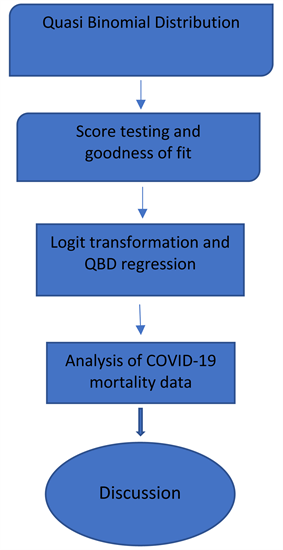
The flowchart in the Appendix outlines the steps of the model developments and the applications.
2. Quasi-Binomial Distribution and
Binomial Score Test of Significance
A discrete random variable Y is said to have a QBD if and only if its probability function is given from [6] as:
(1)
for
and zero otherwise and where
,
. It reduces to the binomial when
. The r.v. Y represents the number of successes in m trials such that the probability for the first success is p and that the probability of success in each of the other trials is
. Thus the probability of success increases or decreases as
is positive or negative and is directly proportional to the number of successes y. All the moments of the QBD are finite and the parameter
has a very substantial effect on the model. The Variance of the QBD is larger or smaller than the variance of the binomial model depending upon
or
. Consul [9] provided a detailed study of the characteristics of the QBD and gave numerous properties and moment based estimation of the model parameters. The mean
of the QBD model (1) is given by
(2)
We shall formulate a
test for testing the binomial model against the QBD alternative. This can be done by testing the null hypothesis
against its negation in the presence of the nuisance parameter p. Moran [9] showed that for such problems the
tests, suggested by Neyman [8], are asymptomatically equivalent to tests using the maximum likelihood estimates.
Let
be n independent random variables where each r. v.
is distributed as a QBD with
. The likelihood function L is given by (3):
(3)
and, its logarithm (4) equals
(4)
To derive the
test statistic for
, the first and second partial derivatives of the log-likelihood function
, evaluated at
, are needed.
All summations are from
to n in the expressions unless stated otherwise. Differentiating the right hand-side of (4) with respect to the model parameters, and setting
we get
(5)
where
.
Setting the second equation in (5) to zero and solving for p yields
(6)
as the maximum likelihood estimator of p under
.
Also, the second partial derivatives are given in (7), (8), (9)
(7)
(8)
(9)
Setting
, the above three equations are obtained in their respective orders as:
(10)
(11)
and,
(12)
Under the null hypothesis
, the
are independent binomial variates. Using the expected values of
and
for binomial variates one can easily see that
.
Denoting
and
we can then show that
(13)
(14)
and
(15)
Equations (13), (14), and (15) are in fact the elements of Fisher’s information matrix when the null hypothesis
is true.
To test the hypothesis
, one can use the statistic
according to Neyman’s methodology [7]. Since p is unknown, we can follow Moran’s suggestion [8] and use the statistic
, where
is any root-n consistent estimator of p. The maximum likelihood estimator
, given in (5) is the simplest such estimator. On substituting
in (4) and on simplifying, we get
(16)
It may be noted that when
, the expression for
reduces to
which is like Fisher’s variance test statistic. From Cox and Hinkley [10],
(17)
The substitution of
for p in (17) gives the functional form of the test statistic, under
, as
(18)
The statistic M2 (18) has an asymptotic (for
) chi-square distribution with one degree of freedom. Accordingly, the above statistic provides a
a binomial score test which is asymptotically optimal against the quasi-binomial alternative.
3. Examples
We shall now consider two examples. In the first example the data sets are binomially distributed and the test statistic M2 does not reject the hypothesis of a binomial distribution and in the second example the test statistic M2 indicates that the data sets are not binomially distributed.
Example 1. Paul [11] discussed a teratological experiment in which pregnant Dutch rabbits were treated with varying doses of a compound. Each litter (group) consisted of a varying number of live fetuses in each rabbit. The number of fetuses in each litter with skeletal of visceral abnormalities were then observed. For illustration, we consider the group, treated with high dose, consisting of
litters which gave the following observations:
Since
and
,
.
To test the null hypothesis H0: The data sets are binomially distributed i.e.
against H1: The data sets are quasi-binomially distributed i.e.
, we compute the following values for (13) to (14) and apply them to (15) and (16).
and
Thus, from (11),
Since
, the null hypothesis cannot be rejected. Thus, we conclude that the data sets are binomially distributed with
.
4. Quasi-Binomial Regression Model
It is well known that the logistic-linear model is a basis for analyzing regression data or the data from designed experiments when the response variable is measured on the binary scale. The purpose of this section is to modify the QBD so that a finite number of concomitant variables may be included which may account for most of the sources of the extra-binomial variation.
Suppose that the ith response
has the QBD given by (1). Also, let
be the values of k explanatory variables associated with the response variable
, where the
matrix is of rank k. We now employ the customary logistic transformation on the binomial parameter p as indicated below”
where,
(19)
where
in the right-hand side of (19) are the regression coefficients which are to be estimated along with the parameter
.
The likelihood function will be given by
(20)
Taking the log of the likelihood function (20) we get the log-likelihood function in (21)
(21)
where the summations are for
to n and
is defined in (19).
Differentiating
, given in (21) partially with respect to
, and
, we have the following system of
equations:
(22)
and
(23)
The second partial derivatives are given by (where
)
and
for
.
The expectations of the negatives of the above second partial derivatives would give the elements of the Fisher’s information matrix. For these we use some results from [9] on inverse moments of the QBD. Thus
(24)
(25)
(26)
where
.
Equations (24), (25), (26) are the elements of Fisher’s information matrix. From [12], and based on the large sample theory of the likelihood estimation, we can establish the asymptotic normality of
; that is
in law. The large sample variance covariance matrix is given by
In testing hypothesis about parameters in a logit model, one generally uses large sample tests. The choice is between the likelihood ratio test and other consistent tests which are asymptotically equivalent to the likelihood ratio test under the null hypothesis [8], in contrast to the likelihood-ratio test which requires fitting the model under both the null and alternative hypotheses). Now, to test the null hypothesis
versus
, the Wald statistic given in (27) is
(27)
In (27)
is the asymptotic variance of
, evaluated under the null hypothesis H0. Under H0, the statistic W has the same asymptotic (for large samples)
distribution as the likelihood ratio statistic. Equivalently,
is rejected whenever the value of
where
is the standard normal deviate for α-level of significance, and
denotes the large sample variance of
, under H0, and after all other parameters are replaced by their maximum likelihood estimates.
5. Applications of the QBD Regression
1) Clinical trial results
One group of 16 pregnant female rats was fed a control diet during pregnancy and lactation and a second group of 16 pregnant female rats was given a diet treated with a chemical. Weil [13] published clinical trial data on the number m of pups alive at 4 days and the number y of pups that died at the end of 21 days lactation period for each litter. The fractions
for the two groups are given below:
Control: 0/13, 0/12, 0/9, 0/9, 0/8, 0/8, 1/13, 1/12,
1/10, 1/10, 1/9, 2/13, 1/5, 2/7, 3/10, 3/10.
Treated: 0/12, 0/11, 0/10, 0/9, 1/11, 1/10, 1/10, 1/9,
1/9, 1/5, 2/9, 3/7, 5/10, 3/6, 7/10, 7/7.
We apply the quasi-binomial regression model to the above data with 16 replications in each group and take
where
and
when the subject is in the control group and
when it is in the treatment group.
The maximum likelihood estimates of
were obtained by simultaneously solving the system of equations.
and
, given in (14) and (15), with the help of NLMIX procedure in SAS (version 9.4). ML estimates are
and
The numbers in the brackets are the large sample standard deviations. Both
and
are highly significant (p-value < 0.001).
2) Example 2: Multiple regression (risk factors associated with COVID 19 case fatality)
The novel coronavirus disease (COVID-19) pandemic affected every country in our world and imposed tremendous strains on the world economies and the health care systems.
During the 2901-2020 year over 5000 research papers have been published and the fundamental aim has been to understand the mechanism of spread of the virus and the main risk factors leading to associated mortality. Many of these reports on the COVID-19 pandemic suggested that the coronavirus was associated with more serious chronic diseases and mortality regardless of country and age. Other reports suggested that those with underlying comorbidities, including obesity, type 2 diabetes, heart, and kidney diseases are at high risk of infection and death. Therefore, there is a need to understand how common comorbidities and other factors are associated with the risk of death due to COVID-19 infection. Our investigation aims at exploring this relationship. Specifically, our fundamental aim is to explore the relationship between the aggregate numbers of deaths among total number of reported COVID-19 cases.
The WHO website [14] provided detailed account of the number of COVID-19 cases by country, which we accessed on December 2-2020. We included in the study the cumulative number of COVID-19 cases and the associated death counts by country as of December 2-2020. We excluded countries that had cumulative counts less than 10,000 cases. We denote the number of cases pe-country by m, and the corresponding deaths denoted by y. The data base has 112 countries, we divided them into regions according to the classification given in data source number [15]. The most referenced risk factors are:
1) X1 = log (percentage of obese persons in a country reported in the year (2018) [17].
2) X2 = log (population density) [18] [19] [20].
3) X3 = log (number of people with colorectal cancer in a country reported in the year (2017) [21].
4) X4 = log (Chronic Kidney Disease-case fatality in a country as reported in (2017) [15] [16].
Note that we used the log (factor) to stabilize the variance. The data are summarized in Table 1.
The histogram of y is given in Figure 1, showing the severe skewness in the distribution.
Figures 2-5 are the box plots of the risk factors. The plot shows that the distributions are evenly distributed among regions, except for X3.
![]()
Table 1. Summary statistics of the COVID-19 cases (m), deaths among cases, and the four covariates.
![]()
Figure 1. Histogram of the number of deaths.
We estimated the average case-fatality rate as:
.
Moreover, the other quantities are given as:
,
,
,
,
.
Hence
, and we therefore reject the binomial hypothesis. We used the SAS NLMIXED procedure to fit the QB regression model. The results are shown in Table 2.
We note that the fitting algorithm produces variance covariance matrix of the estimated regression parameters (not shown here).
The Nonlinear Mixed Model procedure (NLMIXED) is an iterative algorithm and its convergence, which can be slow, depends heavily on the starting.
![]()
Table 2. Results of the quasi-binomial regression for the COVID-19 case fatality data.
6. Discussion
For observed data sets which exhibit variation greater than what is expected under the hypothesized model, the researchers often try to determine the sources of this phenomenon which is known as over-dispersion. There are three broad categories of such sources of over dispersion: 1) genuine or significant over-dispersion or under-dispersion which may be accounted for by generalizations of the known distribution, 2) the apparent over-dispersion is due to some outliers, which may be detected by residual analysis by some other diagnostic method, 3) poor choice of some of the explanatory variables. Therefore, it seems appropriate that one should apply a model which includes a dispersion parameter as well as a reasonable number of carefully chosen covariates and variates. The fitting of the QBD regression model can be tricky, and one may adopt one of the algorithms described in [22] and [23].
Acknowledgements
The authors thank anonymous reviewers for their constructive comments.
Appendix: Flow Chart for the Manuscripts