Temporal Model for Dengue Disease with Treatment

Laurencia Ndelamo Massawe^1*, Estomih S. Massawe¹, Oluwole D. Makinde²

¹Mathematics Department, University of Dar es Salaam, Dar es Salaam, Tanzania.
²Faculty of Military Science, Stellenbosch University, Saldanha, South Africa.

DOI: 10.4236/aid.2015.51003                

Abstract

This paper examines the effect of treatment of Dengue fever disease. A non linear mathematical model for the problem is proposed and analysed quantitatively using the stability theory of the differential equations. The results show that the disease-free equilibrium point is locally andglobally asymptotically stable if the reproduction number (R₀) is less than unity. The additive compound matrices approach is used to show that the dengue fever model’s endemic equilibrium point is locally asymptotically stable when trace, determinant and determinant of second additive compound matrix of the Jacobian matrix are all negative. However, treatment will have a control of dengue fever disease. Numerical simulation of the model is implemented to investigate the sensitivity of certain key parameters on the dengue fever disease with treatment.

Keywords

Dengue Fever Disease, Treatment of Dengue Fever Disease, Equilibrium Stability, Reproduction Number, Sensitivity Index

1. Introduction

Dengue is a vector borne disease transmitted to humans by the bite of an infected female Aedes mosquito [1] . Dengue fever (DF) also known as break-born fever is a mosquito born infection that causes a severe flu-like illness, caused by any one of the four closed related dengue viruses transmitted by female mosquitoes, i.e. DEN-1, DEN-2, DEN-3 and DEN-4. The first recognized Dengue epidemics occurred almost simultaneously in Asia, Africa, and North America in the 1780s, shortly after the identification and naming of the disease in 1779. It has spread especially in the tropical and sub tropical regions around the world, and nowadays is a disease widely found in urban and semi-urban areas, ([2] ). Mathematical modelling is the interesting tool for understanding epidemiological diseases and for proposing effective strategies to fight them ([3] ). The mathematical model of dengue transmission is a multi-population model that captures the transmission dynamics between host (human) and vector (mosquito) taking into account the four strains of dengue virus and the cross infections. Various models have been proposed to study factors on the transmission dynamics and control the spread of dengue fever disease ([2] -[10] , studied a dengue model by evaluating and analysing the sensitivity indices of the reproduction number in order to determine the relative importance of the model parameters in the disease transmission. So far no one considered a dynamical system that incorporates the effects of treatment in dengue fever disease model. In this paper, it is therefore intended to analyse a model which will include treatment. Thus, we study and analyse a non linear mathematical model showing the effect of treatment on the transmission of dengue fever disease in the population.

2. Model Formulation

A non linear mathematical model is formulated and analysed showing the effect of treatment of Dengue fever disease. The basic reproduction number and stability of equilibrium points are analysed qualitatively. Sensitivity analysis of parameters and numerical simulations are performed. The total human population at any time t will be denoted by The total population is subdivided into four sub-populations namely; Susceptibles, Infectives, Treated and Resistant.

Thus

where―represent human population.

There are three other state variables, related to the female mosquitoes, indexed by:

―Aquatic phase (that includes the egg, larva and pupa stages);

―Susceptibles (mosquitoes that are able to contract the disease);

―Infectives (mosquitoes capable of transmitting the disease to human).

In formulating the model, the following assumptions are considered:

i) Total human population is constant at any time t, i.e.,

ii) The population is homogeneous, which means that every individual of a compartment is homogeneously mixed with the other individuals,

iii) Immigration and emigration are not considered,

iv) Each vector has an equal probability to bite any host,

v) Humans and mosquitoes are assumed to be born susceptible i.e. there is no natural protection,

vi) The coefficient of transmission of the disease is fixed and does not vary seasonally,

vii) For the mosquito there is no resistant phase, due to its short lifetime, ([10] ).

Considering the above assumptions, we then have the following

Schematic model flow diagram for dengue fever disease with treatment:

From Figure 1 flow diagram, the model will be governed by the following equations:

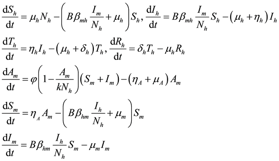(1)

where

Figure 1. Model flow diagram for dengue fever disease with treatment.

, , , , , , , for all.

3. Model Analysis

The model system of Equation (1) will be analysed qualitatively to get a better understanding of the effects of treatment of Dengue fever disease. The basic Reproduction number which governs elimination or persistence of Dengue fever disease will be determined and studied.

3.1. Disease Free Equilibrium (DFE)

For the disease free equilibrium, it is assumed that there is no infection for both populations of human and mosquitoes i.e. and, denoted by “”. Thus of the model system (1) is obtained as

(2)

3.2. The Basic Reproduction Number, “R₀”

The basic reproduction number, denoted by, is defined as the average number of secondary infections that occurs when one infective individual is introduced into a completely susceptible population ([11] ).

The basic reproduction number of the model (1) is calculated by using the next generation matrix of an ODE ([11] ). Using the approach of ([11] ). is obtaining by taking the largest (dominant) eigenvalue (spectral radius) of

where, is the rate of appearance of new infection in compartment, is the transfer of individuals out of the compartment by all other means and is the disease free equilibrium.

Using the linearization method, the associated matrix at DFE is given by

This implies that

With, we have

or

The transfer of individuals out of the compartment is given by

Using the linearization method, the associated matrix at DFE is given by

This gives with

Therefore

(3)

The eigenvalues of the Equation (3) are given by

This gives

It follows that the Reproductive number which is given by the largest eigenvalue for model system (1) with treatment denoted by is given by

(4)

where.

If, the disease cannot invade the population and the infection will die out over a period of time, and also, if, then an invasion is possible and infection can spread through the population. Generally, the larger the value of, the more severe, and possibly widespread the epidemic will be, ([10] ).

3.3. Sensitivity Analysis of Model Parameters

In order to determine how best human mortality due to dengue fever is reduced, we calculate the sensitivity indices of the reproduction number to each parameter in the model using the approach of ([11] ). These indices tell us which parameters have high impact on and should be targeted by intervention strategies. Also Sensitivity indices allow us to measure the relative change in a variable when a parameter changes. The normalized forward sensitivity index of a variable with respect to a parameter is the ratio of the relative change in the variable to the relative change in the parameter. When the variable is a differentiable function of the parameter, the sensitivity index may be alternatively be defined using partial derivatives.

Definition 1: The normalized forward sensitivity index of “”, that depends differentiable on a parameter “”, is defined as ([12] )

(5)

As we have an explicit formula for in the Equation (5), we derive an analytical expression for the sensitivity of as to each of parameters involved in. For example, using the set of estimated parameter values given as, , , , , , , , , the sensitivity indices of with respect to and are given by and respectively. Otherindices, , , , , , and are obtained following the same method and tabulated as follows:

The parameters are ordered from most sensitive to the least.

Interpretation of Sensitivity Indices

From Table 1 generally it shows that the parameters, , , , and each increases keeping other parameters constant they increase the value of implying that they increase the endemicity of the disease as they have positive indices. While the parameters, , and when each increases while keeping the other parameters constant they decrease the value of implying that they decrease the endemicity of the disease as they have negative indices.

But individually, the most sensitive parameter is the average daily biting (per day), followed by maturation rate from larvae to adult (per day), transmission probability from (per bite), number of larvae per human, transmission probability from (per bite), number of eggs at each deposit per capita (per day), then average lifespan of humans (per day), natural mortality of larvae (per day), mean viremic period (per day), and finally the least sensitive parameter is the average lifespan of adult mosquitoes (per day).

3.4. Local Stability of Disease Free Equilibrium Point

To determine the local stability of the disease free equilibrium, the variation matrix of the model system (1) corresponding to the disease free is obtained as

(6)

where

Therefore the stability of the disease free equilibrium point can be clarified by studying the behaviour of in which for local stability of DFE we seek for its all eigenvalues to have negative real parts. It follows that, the characteristic function of the matrix (6) with being the eigenvalues of the Jacobian matrix, by using Mathe- matica software the Jacobian matrix has the following eigenvalues:

Table 1. Sensitivity Indices of model parameters to.

when is not a real number.

The other eigenvalues are given as

when is not a real number,

when is not a real number, and finally

when is not a real number.

Hence under certain conditions the system is stable since all the seven eigenvalues are negative. These imply that at the Disease Free Equilibrium point is locally asymptotically stable, i.e. Dengue infection can be eliminated from the population.

3.5. Global Stability of Disease Free Equilibrium Point

In this subsection, we analyse the global behaviour of the equilibria for system (1). The following theorem provides the global property of the disease free equilibrium of the system. The results are obtained by means of Lyapunov function. In choosing the Lyapunov function the idea of [13] is used.

Theorem 1: If, then the infection-free equilibrium is globally asymptotically stable in the interior of.

Proof:

To establish the global stability of the disease-free equilibrium, we construct the following Lyapunov function:

(7)

Calculating the time derivative of along (7), we obtain

Then substituting and from system (1), we get

where

It follows that

or

which is equivalent to

But

or

(9)

Substituting (9) into (8) yields

Therefore

Thus, is negative if, and if and only if is reduced to the disease-free equilibrium. Consequently, the largest compact invariant set in when is the singleton. Hence, by LaSalle’s invariance principle it implies that “” is globally asymptotically stable in ([14] ).This completes the proof.

3.6. Existence and Local Asymptotic Stability of Endemic Equilibrium

Since we are dealing with presence of dengue fever disease in human population, we can reduce system (1) to a 3-dimensional system by eliminating, , and respectively, in the feasible region. The values of can be determined by setting to obtain

(10)

The endemic equilibrium of the system (10) is given by. It is obtained by setting the right hand side of each equation of the system (10) equal to zero which exist for. Thus, we have

(11)

(12)

(13)

3.6.1. Existence of Endemic Equilibrium

For the existence and uniqueness of endemic equilibrium, the conditions or i.e. or or, must be satisfied by using the idea of ([15] ).

Adding Equations (11)-(13) above, we have

or

But from (13) above

It follows that

or

Consequently

Then

This imply that

and

meaning that

Thus, the endemicity of the disease exists since, , and.

3.6.2. Local Stability of the Endemic Equilibrium

In order to analyse the stability of the endemic equilibrium, the additive compound matrices approach is used, using the idea of ([16] ).

If then the host-vector model Equations (11)-(13) has a unique endemic equilibrium given by in, with

(14)

(15)

(16)

Local stability of the endemic equilibrium point is determined by the variational matrix of the nonlinear system (9) corresponding to as

(17)

The following lemma was stated and proved by [17] , to demonstrate the local stability of endemic equilibrium point.

Lemma 1: Let be the variational matrix corresponding to. If, and are all negative, then all eigenvalues of have negative real parts.

Using the above Lemma, we will study the stability of the endemic equilibrium.

Theorem 2: If the endemic equilibrium of the model (10) is locally asymptotically stable in.

Proof:

From the Jacobian matrix in (17), we have

Thus,

Using Mathematica software, we get

Hence trace and determinant of the Jacobian matrix are all negative.

The second additive compound matrix is obtained from the following lemma.

Lemma 2: Let and be subset of. The entry of is the coefficient of in the expansion of the determinant of the sub matrix of indexed by row in and column in.

Proof:

The sub matrix of is given as

The sub matrix of indexed by rows and columns in is given by

The coefficient of in the determinant of this matrix is and thus the entry of is.

Other entries were done following the same method and to obtain

Thus

Using Mathematica software, we get

Therefore.

Thus, from the lemma 1, the endemic equilibrium of the model system (10) is locally asymptotically stable in.

4. Numerical Simulations

Here, we illustrate the analytical results of the study by carrying out numerical simulations of the model system (1) using the set of estimated parameter values given as shown below.

(18)

Figure 2 shows that the proportion of Dengue fever disease infectives, treated and recovery proportion of Dengue fever disease all plotted against the proportion of susceptible population. This shows the dynamic behaviour of the endemic equilibrium of the model system (1) using the parameter values in (18) for different initial

Figure 2. Variation of proportion of Dengue fever disease infective population, treated population and recovery population of Dengue fever disease against proportion of susceptibles population.

starting values in three cases as shown below [12] .

The equilibrium point of the endemic equilibrium was obtained as

It is observed from Figure 2 that for any starting initial value, the solution curves tend to the equilibrium. Therefore we conclude that the model system (1) is globally stable about this endemic equilibrium point for the parameters displayed in (18).

Figures 3(a)-(d) show the variation of population in different classes, human susceptibles, treated human infective, dengue fever patient for different values of (average daily biting (per day)).

From Figure 3(a), it is observed that proportion of susceptible human population decreases in time slightly before reaching its equilibrium position due to treatment. Therefore, infection becomes less endemic in the pop-

(a) (b)(c) (d)

Figure 3. Distribution of population with time in all classes of human and mosquito, Variation of proportion of dengue fever disease infected population ,treated human population and Dengue Fever Patient for different values of (b) (average daily biting (per day)).

ulation. The proportion of Dengue fever disease infectives decreases in time then reaches equilibrium due to the increase in the number of population getting treatment. Moreover treated infectives increase and then decrease due to infected population moving to other classes, and then also recovery population increases in time as more population are treated. Furthermore infected mosquitoes decrease when the recovery population increases. Mosquito susceptible and aquatics increase with time and reaches its equilibrium point due to its short life span.

From Figure 3(b), it is observed that there is increase in population of dengue fever disease infectives as the value of increased. If no treatment, large population will die within a very short period of time.

From Figure 3(c), it is seen that when biting rate increases, the proportional of treated infectives increases and reaches its equilibrium point.

From Figure 3(d), it is observed that when biting rate increase, the proportion of Dengue fever disease increases with time. Therefore protective measures should be taken on board.

Figure 4(a) and Figure 4(b) shows the variation of proportion of dengue fever treated population and recovery population for different values of (Rate at which dengue fever infected individuals progress for treatment).

From Figure 4(a), it is observed that when treatment is increased, the treated proportion decreases due to treated individuals leaving the class. Moreover when there is no treatment, treated infectives increase and reaches equilibrium due to the decrease of population implying that death rate is high due to lack of treatment.

From Figure 4(b), it is observed that when there is no treatment, i.e., the dengue fever population decreases. This implies that, death rate increases since there is no treatment. However, when treatment is in progress, a significant increase in the dengue fever recovery (patients) is observed. This also implies that

(a) (b)

Figure 4. Variation of proportion of dengue fever treated population and recovery population for different values of (Rate at which dengue fever infected individuals progress for treatment).

patients get treatment which prolongs their lives.

5. Discussion and Conclusion

5.1. Discussion

A nonlinear mathematical model has been analysed to study the effect of treatment on the dengue fever disease. The analysis of the model shows that the disease-free equilibrium is locally asymptotically stable by next generation method, which involves the computation of basic reproduction number less than unity and unstable at reproduction number greater than unity. Then also by using Lyapunov method the disease-free equilibrium point is globally asymptotically stable when and unstablewhen. Furthermore there exists endemic equilibrium point, that is locally asymptotically stable when, and are all negative, then all eigenvalues of have negative real parts, where is the variational matrix corresponding to.

Numerical results are provided to illustrate the analytical results. Sensitivity analysis shows that the average daily biting (per day) is the most sensitive parameter on and the least sensitive is the average lifespan of adult mosquitoes (per day).

In numerical simulation it is observed that the increase of average daily biting (per day), tends to increase the number of infectious individual in the population. But the absence of average daily biting (per day), the infectious population is lowered and the disease can be eradicated. Moreover the increase of treatment will result the reduction of infected proportion as infected proportion population will move to other class, on the other hand when treatment is applied majority of infectious will be observed, as treatment will prolong the life of individual, but with no treatment infectious will be reduced because majority will die and will reach at equilibrium point. From this indicate that there is much work to be done to eradicate the disease by driving reproduction number to be less than unity. Thus the best thing to do is spraying pesticides to kill mosquitoes or sterile male mosquitoes as biological control.

5.2. Conclusion

A compartmental model for Dengue fever disease was presented, a model based on two populations, humans and mosquitoes with treatment. Simulation shows that on the application of treatment, the number of death is reduced. It has been proved algebraically that, if a constant minimum level of a treatment is applied, it is possible to maintain the basic reproduction number below unity, and the infected humans were smaller.

NOTES

^*Corresponding author.

Conflicts of Interest

The authors declare no conflicts of interest.

References

[1]	Semenza, J.C. and Menne, B.B. (2009) Climate Change and Infectious Diseases in Europe. The Lancet Infectious Diseases, 9, 365-375. http://dx.doi.org/10.1016/S1473-3099(09)70104-5
[2]	Rodrigues, H.S., Monteiro, M.T.T., Torres, D.F.M and Zinober, A. (2011) Dengue Disease, Basic Reproduction Number and Control. International Journal of Computer Mathematics, 1-13.
[3]	Lenhart, S. and Workman, J.T. (2007) Optimal Control Applied to Biological Models. Chapman& Hall/CRC Mathematical and Computational Biology Series, Chapman & Hall/CRC, Boca Raton.
[4]	Chikaki, E. and Ishikawa, H. (2009) A Dengue Transmission Model in Thailand Considering Sequential Infections with All Four Serotypes. J Infect Devctries, 3, 711-722.
[5]	Thome, R.C., Yang, H.M. and Esteva, L. (2010) Optimal Control of Aedes aegypti Mosquitoes by the Sterile Insect Technique and Insecticide. Mathematical Biosciences, 223, 12-23. http://dx.doi.org/10.1016/j.mbs.2009.08.009
[6]	Rodrigues, H.S., Monteiro, M.T.T. and Torres, D.F.M. (2010) Insecticide Control in a Dengue Epidemics Model. In: Simos, T., Ed., AIP Conference of Proceedings of the Numerical Analysis and Applied Mathematics, 1281, 979-982.
[7]	Centers for Disease Control and Prevention (2011) Division of Vector Borne and Infectious Diseases, Prevention, How to Reduce Your Risk of Dengue Infection. http://www.cdc.gov/Dengue/prevention/index.html.
[8]	Rodrigues, H.S., Monteiro, M.T.T. and Torres, D.F.M. (2012) Modeling and Optimal Control Applied to a Vector Borne Disease. International Conference on Computational and Mathematical Methods in Science and Engineering, CMMSE, 2012, 1063-1070.
[9]	Rodrigues, H.S., Monteiro, M.T.T. and Torres, D.F.M. (2013) Bioeconomic Perspectives to an Optimal Control Dengue Model. International Journal of Computer Mathematics, 2013.
[10]	Rodrigues, H.S., Monteiro, M.T.T. and Torres, D.F.M. (2013) Sensitivity Analysis in a Dengue Epidemiological Model. Conference Papers in Mathematics, 2013.
[11]	van den Driessche, P. and Watmough, J. (2002) Reproduction Numbers and Sub-Threshold Endemic Equilibria for Compartmental Models of Disease Transmission. Mathematical Biosciences, 180, 29-48. http://dx.doi.org/10.1016/S0025-5564(02)00108-6
[12]	Ratera, S., Massawe, E.S. and Makinde, O.D. (2012) Modelling the Effect of Screening and Treatment on Transmission of HIV/AIDS Infection in Population. American Journal of Mathematics and Statistics, 2, 75-88. http://dx.doi.org/10.5923/j.ajms.20120204.03
[13]	Ozair, M., Lashari, A.A., Jung, I.H., Seo, Y.I. and Kim, B.N. (2013) Stability Analysis of a Vector-Borne Disease with Variable Human Population. Research Article Stability, 2013, 1-12
[14]	LaSalle, J.P. (1976) The Stability of Dynamical Systems. Regional Conference Series in Applied Mathematics, SIAM, Philadelphia.
[15]	Tumwiine, J., Mugisha, J.Y.T. and Luboobi, L.S. (2007) A Mathematical Model for the Dynamics of Malaria in a Human Host and Mosquito Vector with Temporary Immunity. Applied Mathematics and Computation, 189, 1953-1965. http://dx.doi.org/10.1016/j.amc.2006.12.084
[16]	Lee, K.S. and Lashari, A.A. (2014) Global Stability of a Host-Vector Model for Pine Wilt Disease with Nonlinear Incidence Rate. Abstract and Applied Analysis, 2014, 1-11
[17]	McCluskey, C.C. and van den Driessche, P. (2004) Global Analysis of Two Tuberculosis Models. Journal of Differential Equations, 16, 139-166. http://dx.doi.org/10.1023/B:JODY.0000041283.66784.3e