Inferences for the Generalized Logistic Distribution Based on Record Statistics ()
1. Introduction
Record values and the associated statistics are of interest and importance in many areas of real life applications involving data relating to meteorology, sport, economics, athletic events, oil, mining surveys and lifetesting. Many authors have studied records and associated statistics. Among them are Ahsanulla [1] [2] , Resnick [3] , Raqab and Ahsanulla [4] , Nagaraja [5] , Arnold et al. [6] [7] , Raqab [8] , Abd Ellah [9] [10] , Sultan and Balakrishnan [11] , Preda and Panaitescu [12] , Mahmoud et al. [13] and Sultan et al. [14] .
Let  a sequence of independent and identically distributed (iid) random variables with cumulitive distribution function
  and probability density function
 . Setting
 we say that
  is a lower record and denoted by
  if
if ,
,
 . For more detail and references see Nagaraja [5] , Ahsanullah [2] and Arnold et al. [7] .
The standard logistic distribution has important uses in describing growth and as a substitute for the normal distribution. It has also attracted interesting applications in the modeling of the dependence of chronic obstructtive respiratory disease prevalence on smoking and age, degrees of pneumoconiosis in coal miners, geological issues, hemolytic uremic syndrome data for children, physicochemical phenomenon, psychological issues, survival time of diagnosed leukemia patients, and weight gain data. A generalized logistic distribution is proposed, based on the fact that the difference of two independent Gumbel distributed random variables has the standard logistic distribution. The generalized logistic distribution (GLD) has received additional attention in estimating its parameters for practical usage see for example Asgharzadeh [15] . The form of the probability density function (pdf) and cumulative distribution function (cdf) of the two parameter generalized logistic distribution denoted by  are given, respectively, by
 (1)
(1)
 (2)
(2)
Here  and
and  are the shape and scale parameters, respectively, the above GLD was originally proposed as a generalization of the logistic distribution by Johnson et al. [16] . For
 , the GLD becomes the standard logistic and it is symmetric. The pdf in (1) has been obtained by compounding an extreme value distribution with a gamma distribution, different estimation procedures can be found in Chen and Balakrishnan [17] .
The rest of the paper is organized as follows. In Section 2, we derive point estimation and the approximate confidence interval based on maximum likelihood estimation. The parametric bootstrap confidence intervals are discussed in Section 3. Section 4 describes Bayes estimates and construction of credible intervals using the MCMC algorithms. Section 5 contains the analysis of a numerical example to illustrate our proposed methods. A simulation studies are reported in order to give an assessment of the performance of the different estimation methods in Section 6. Finally we conclude with some comments in Section 7.
2. Maximum Likelihood Estimation
Suppose that  be the lower record values of size
  from the generalized logistic distribution
 . The likelihood function for observed record
  was given by see Arnold et al. [7]
 (3)
(3)
where  and
and  are given respectively, by (1) and (2), the likelihood function can be obtained by substituting from (1) and (2) in (3) and written as
 (4)
(4)
The natural logarithm of the likelihood function (4) is given by
 (5)
(5)
Differentiating (5) with respect to  and
and  and equating the results to zero, we obtain the likelihood equations for the parameters
  and
and  as
as
 (6)
(6)
 (7)
(7)
From (6), the maximum likelihood estimate (MLE) of  say
say , can be obtained as
 (8)
(8)
The MLE of the  say
say  can be obtained by solving the non-linear likelihood equation
 (9)
(9)
Therefore,  can be obtained as the solution of the non-linear equation in the form
 , (10)
where
 (11)
(11)
Since  is a fixed point solution of non-linear equation (9), therefore, it can be obtained by using a simple iterative scheme as follows
 (12)
(12)
where  is the
  iterate of
 . The iteration procedure should be stopped when
  is sufficiently small. Once we obtain
  from (9), and the MLE of
  say
say  becomes
 (13)
(13)
The asymptotic variance—covariance matrix of the maximum likelihood estimates for the two parameters  and
and  is the inverse of the Fisher information matrix after ignoring the expectation operators as following
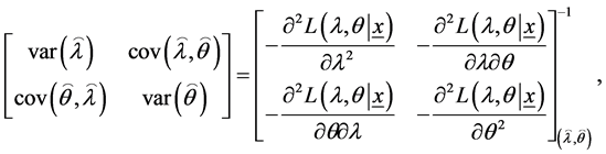 (14)
(14)
with
 (15)
(15)
 (16)
(16)
 (17)
(17)
where
 (18)
(18)
 (19)
(19)
The asymptotic normality of the MLE can be used to compute the approximate confidence intervals for parameters  and
and . Therefore,
  confidence intervals for parameters
 , and
, and  become, respectively, as
 (20)
(20)
where  is the percentile of the standard normal distribution with right-tail probability
 .
.
3. Bootstrap Confidence Intervals
In this section, we propose to use confidence intervals based on the parametric bootstrap methods 1) percentile bootstrap method (Boot-p) based on the idea of Efron [18] ; 2) bootstrap-t method (Boot-t) based on the idea of Hall [19] . The algorithms for estimating the confidence intervals using both methods are illustrated as follows.
3.1. Percentile Bootstrap Method
Algorithm 1
Step 1. From the original data  compute the ML estimates of the parameters
  and
and
 by (13) and (9).
Step 2. Use  and
and  to generate a bootstrap sample
 .
.
Step 3. As in Step 1, based on  compute the bootstrap sample estimates of
  and
and , say
, say  and
and .
.
Step 4. Repeat Steps 2-3  times representing
  bootstrap MLE’s of
  and
and  based on
  different bootstrap samples.
Step 5. Arrange all  and
and , in an ascending order to obtain the bootstrap sample
 (where
 ,
, ).
).
Let  be the cumulative distribution function of
 . Define
  for given
 .
.
The approximate bootstrap  confidence interval of
  is given by
 . (21)
3.2. Bootstrap-t Method
Algorithm 2
Step 1. From the original data  compute the ML estimates of the parameters
  and
and
 by equations (13) and (9).
Step 2. Using  and
and  generate a bootstrap sample
  Based on these data, compute the bootstrap estimate of
  and
and , say
, say  and
and  and following statistics

where  and
and  are obtained using the Fisher information matrix.
Step 3. Repeat Step 2, N boot times.
Step 4. For the  and
and  values obtained in Step 2, determine the upper and lower bounds of the
  confidence interval of
  and
and  as follows: let
  be the cumulative distribution function of
  and
and . For a given
 , define

Here also,  and
and  can be computed as same as computing the
  and
and .
.
The approximate  confidence interval of
  and
and  are given by
 (22)
(22)
4. Bayes Estimation Using MCMC
In Bayesian approach, the performance depends on the prior information about the unknown parameters and the loss function. The prior information can be expressed by the experimenter, who has some beliefs about the unknown parameters and their statistical distributions. This section describes Bayesian MCMC methods that have been used to estimate the parameters of the generalized logistic distribution (GLD). The Bayesian approach is introduced and its computational implementation with MCMC algorithms is described. Gibbs sampling procedure [20] [21] and the Metropolis-Hastings (MH) algorithm [22] [23] are used to generate samples from the posterior density function and in turn compute the Bayes point estimates and also construct the corresponding credible intervals based on the generated posterior samples. By considering model (1), assume the following gamma prior densities for  and
and  as
as
 (23)
(23)
and
 (24)
(24)
The joint prior density of  and
and  can be written as
 (25)
(25)
Based on the likelihood function of the observed sample is same as (4) and the joint prior in (25), the joint posterior density of  and
and  given the data, denoted by
 , can be written as
 (26)
(26)
therefore, the Bayes estimate of any function of  and
and  say
say , under squared error loss function is
 (27)
(27)
The ratio of two integrals given by (27) cannot be obtained in a closed form. In this case, we use the MCMC algorithm to generate samples from the posterior distributions and then compute the Bayes estimator of  under the squared errors loss (SEL) function. For more details about the MCMC methods see, for example, Rezaei et al. [24] and Upadhyaya and Gupta [25] .
4.1. MCMC Algorithm
The Markov chain Monte Carlo (MCMC) algorithm is used for computing the Bayes estimates of the parameters  and
and  under the squared errors loss (SEL) function. We consider the Metropolis-Hastings algorithm, to generate samples from the conditional posterior distributions and then compute the Bayes estimates. The Metropolis-Hastings algorithm generate samples from an arbitrary proposal distribution (i.e. a Markov transition kernel). The expression for the joint posterior can be obtained up to proportionality by multiplying the likelihood with the joint prior and this can be written as
 (28)
(28)
from (28), the conditional posteriors distribution of parameter  can be computed and written, by
 (29)
(29)
Therefore, the conditional posteriors distribution of parameter , is gamma with parameters
  and
and
 and, therefore, samples of
  can be easily generated using any gamma generating routine.
The conditional posteriors distribution of parameter  can be written as
 (30)
(30)
The conditional posteriors distribution of parameter  Equation (30) cannot be reduced analytically to well known distributions and therefore it is not possible to sample directly by standard methods, but the plot of it (see Figure 1) show that it is similar to normal distribution. So to generate random numbers from this distribution, we use the Metropolis-Hastings method with normal proposal distribution. The choice of the hyper parameters
  and
and  which make (30) close to the proposal distribution and obviously more convergence of the MCMC iteration. We propose the following MCMC algorithm to draw samples from the posterior density functions; and in turn compute the Bayes estimates and also, construct the corresponding credible intervals.
Algorithm 3
Step 1.
 .
.
Step 2. Generate  from gamma distribution
Step 3. Generate  from
from  using (MH) algorithm in [22] [23] .
Step 4. Compute  and
and .
.
Step 5. Repeat Steps 2-4  times.
Step 6. Obtain the Bayes estimates of  and
and  with respect to the SEL function as


Step 7. To compute the credible intervals of  and
and ,
,  order and
  as
as 
and . Then the
  symmetric credible intervals of
  and
and  become
 (31)
(31)
5. Numerical Computations
To illustrate the estimation results obtained in the above sections, consider the first seven lower record values simulated from a two-parameter generalized logistic distribution (1) with shape and scale parameters, respectively

Figure 1. Posterior density function of  given
given .
.
tively,  and
and , as follows: 1.0509, 0.0780, −0.1271, −0.1892, −0.6437, −1.0886, −1.1212. Based on these lower upper record values, we compute the approximate MLEs, Bootstrap (Boot-p, Boot-t) and Bayes estimates of
  and
and  using MCMC algorithm, we assume that informative priors
  and
and  on both
  and
and . The density function of
  given in (30) is plotted Figure 1. It can be approximated by normal distribution function as mentioned in Subsection 4.1. Also the 95%, approximate maximum likelihood estimation (AMLE) confidence intervals, Bootstrap confidence intervals and approximate credible intervals based on the MCMC samples are computed. The results are given in Table1 Figure 2 and Figure 3 plot the MCMC output of
  and
and , using 10 000 MCMC samples (dashed line represent means and red lines represent lower and upper bounds of 95% probability intervals). The plot of histogram of
  and
and  generated by MCMC method are given in Figure 4 and Figure 5. This was done with 1000 bootstrap sample and 10,000 MCMC sample and discard the first 1000 values as “burn-in”.
6. Simulation Study and Comparisons
In this section, we conduct some numerical computations to compare the performances of the different estimators proposed in the previous sections. Monte Carlo simulations were performed utilizing 1000 lower record samples from a two-parameter generalized logistic distribution (GLD) for each simulation. The mean square error (MSE) is used to compare the estimators. The samples were generated by using ,
,  , with different sample of sizes
 . For computing Bayes estimators, we used the non-informative gamma priors for both the parameters, that is, when the hyper parameters are 0. We call it prior 0:
 . Note that as the hyper parameters go to 0, the prior density becomes inversely proportional to its argument and also becomes improper. This density is commonly used as an improper prior for parameters in the range of 0 to infinity, and this prior is not specifically related to the gamma density. For computing Bayes estimators, other than prior 0, we also used informative prior, including prior 1,
  ,
,  ,
,  and
and , also we used the squared error loss (SEL) function to compute the Bayes estimates. We also computed the Bayes estimates and 95% credible intervals based on 10,000 MCMC samples and discard the first 1000 values as “burn-in”. We report the average Bayes estimates, mean squared errors (MSEs) and coverage percentages. For comparison purposes, we also computed the MLEs and the 95% confidence intervals based on the observed Fisher information matrix. Finally, we used the same 1000 replicates to compute different estimates Tables 2-5 report the results based on MLEs and the Bayes estimators (using MCMC algorithm) on both
  and
and .
.
7. Conclusions
The main aim of this paper is study the estimate the parameters of the generalized Logistic distribution using the Bootstrap, MCMC algorithms and comparing them through numerical example and simulation study. There are many authors have studied classic Bayesian methods, for example, Amin [26] discussed Bayesian and nonBayesian estimation from Type I generalized Logistic distribution based on lower record values, Aly and Bleed

Figure 4. Histogram of  generated by MCMC method.

Figure 5. Histogram of  generated by MCMC method.

Table 1. Results obtained by MLE, Bootstrap and MCMC method of  and
and .
.
Table 2. Average values of the different estimators and the corresponding MSEs. when .
.
Note: The first figure represents the average estimates, with the corresponding MSEs reported below it in parentheses.
Table 3. The average confidence lengths relative estimate of parameters and the corresponding coverage percentages when .
.
Note: The first figure represents the average confidence lengths, with the corresponding coverage percentages reported below it in parentheses.
Table 4. Average values of the different estimators and the corresponding MSEs when .
.
Note: The first figure represents the average estimates, with the corresponding MSEs reported below it in parentheses.
Table 5. The average confidence lengths relative estimate of parameters and the corresponding coverage percentages when .
.
Note: The first figure represents the average confidence lengths, with the corresponding coverage percentages reported below it in parentheses.
[27] presented Bayesian estimation for the generalized Logistic distribution Type-II censored accelerated life testing. In this paper Bayesian estimation for the parameters of the generalized logistic distribution (GLD) are computed based on the lower record values using MCMC method. We assume the gamma priors on the unknown parameters and provide the Bayes estimators under the assumptions of squared error loss functions (SEL). The Metropolis-Hastings (MH) algorithm from the MCMC method is used for computing Bayes estimates. It has been noticed that1) From the results obtained in Tables 2-5, it can be seen that the performance of the Bayes estimators with respect to the non-informative prior (prior 0) is quite close to that of the MLEs, as expected. Thus, if we have no prior information on the unknown parameters, then it is always better to use the MLEs rather than the Bayes estimators, because the Bayes estimators are computationally more expensive.
2) Tables 2-5 report the results based on non-informative prior (prior 0) and informative prior, (prior 1) also in these case the results based on using MH algorithm are quite similar in nature when comparing the Bayes estimators based on informative prior clearly shows that the Bayes estimators based on prior 1 perform better than the MLEs, in terms of MSEs.
3) From Tables 2-5, it is clear that the Bayes estimators based on informative prior perform much better than noninformative prior and the MLEs in terms of MSEs.
Acknowledgements
The author would like to express their thanks to the editor, assistant editor and referees for their useful comments and suggestions on the original version of this manuscript.