Automatic Variable Selection for High-Dimensional Linear Models with Longitudinal Data ()
Keywords: Variable Selection; Diverging Number of Parameters; Longitudinal Data; Quadratic Inference Functions; Generalized Estimating Equation
1. Introduction
Longitudinal data arise frequently in biomedical and health studies in which repeated measurements form the same subject are correlated. A major aspect of longitudinal data is the within subject correlation among the repeated measurements. Ignoring this within subject correlation causes a loss of efficiency in general problems. One of the commonly used regression methods for analyzing longitudinal data is generalized estimating equations (Liang and Zeger, [1]). Generalized estimating equations (GEE) using a working correlation matrix with nuisance parameters estimate regression parameters consistently even when the correlation structure is misspecified. However, under such misspecification, the estimator can be inefficient. For this reason, Qu et al. [2] proposed a method of quadratic inference functions (QIF). It avoids estimating the nuisance correlation structure parameters by assuming that the inverse of working correlation matrix can be approximated by a linear combination of several known basis matrices. The QIF can efficiently take the within subject correlation into account and is more efficient than the GEE approach when the working correlation is misspecified. The QIF estimator is also more robust against contamination when there are outlying observations (Qu and Song, [3]).
High-dimensional longitudinal data, which consist of repeated measurements on a large number of covariates, arise frequently from health and medical studies. Thus, it is important for statisticians to develop a new statistical methodology and theory of variable selection and estimation for high-dimensional longitudinal data, which can reduce the modeling bias. Generally speaking, most of the variable selection procedures are based on penalized estimation using penalty functions. Such as,  penalty (Frank and Friedman, [4]), LASSO penalty (Tibshirani, [5]), SCAD penalty (Fan and Li, [6]), and so on. In the longitudinal data framework, Pan [7] proposed an extension of the Akaike information criterion (Akaike, [8]) by applying the quasi-likelihood to the GEE, assuming independent working correlation. Wang and Qu [9] developed a Bayesian information type of criterion (Schwarz, [10]) based on the quadratic inference functions. Fu [11] applied the bridge penalty model to the GEE and Xu et al. [12] introduced the adaptive lasso for the GEE setting, and references therein. These methods are able to perform variable selection and parameter estimation simultaneously. However, most of the theory and implementation is restricted to a fixed dimension of parameters.
Despite the importance of variable selection in high-dimensional settings (Fan and Li, [13]; Fan and Lv, [14]), variable selection for longitudinal data that take into consideration the correlation information is not well studied when the dimension of parameters diverges. In this paper we use the smooth-threshold generalized estimating equation based on quadratic inference functions (SGEE-QIF) to the high-dimensional longitudinal data. The proposed procedure automatically eliminates the irrelevant parameters by setting them as zero, and simultaneously estimates the nonzero regression coefficients by solving the SGEE-QIF. Compared to the shrinkage methods and the existing research findings reviewed above, our method offers the following improvements: 1) the proposed procedure avoids the convex optimization problem; 2) the proposed SGEE-QIF approach is flexible and easy to implement; 3) the proposed method is easy to deal with the longitudinal correlation structure and extend the estimating equations approach to high-dimensional longitudinal data.
The rest of this paper is organized as follows. In Section 2 we first propose variable selection procedures for high-dimensional linear models with longitudinal data, and asymptotic properties of the resulting estimators. In Section 3 we give the computation of the estimators as well as the choice of the tuning parameters. In Section 4 we carry out simulation studies to assess the finite sample performance of the method. Some assumptions and the technical proofs of all asymptotic results are provided in the Appendix.
2. Automatic Variable Selection Procedure
2.1. Model and Notation
We consider a longitudinal study with  subjects and
  observations over time for the
  th subject
 for a total of
  observation. Each observation consists of a response variable
  and a covariate vector
  taken from the
  th subject at time
 . We assume that the full data set
 is observed and can be modelled as
 (2.1)
(2.1)
where  is a
is a  vector of unknown regression coefficients, and
  diverging as the sample size increases.
  is random error with
 . In addition, we give assumptions on the first two moments of the observations
 , that is,
  and
and , where
  is a known variance function.
2.2. Quadratic Inference Functions
Denote  and write
  in a similar fashion. Following Liang and Zeger [1], a GEE can be used to estimate the regression parameters,
  ,
,
 (2.2)
(2.2)
where  is the covariance matrix of
 . The matrix
  is often modelled as
 , where
  is a diagonal matrix representing the variance of
 , that is,
  ,
,  is a common working correlation depending on a set of unknown nuisance parameters
 . Based on the estimation theory associated with the working correlation structure, the GEE estimator of the regression coefficient proposed by Liang and Zeger [1] is consistent if consistent estimators of the nuisance parameters
  can be obtained. For suggested methods for estimating
 , see Liang and Zeger [1]. However, even in some simple cases, consistent estimators of
  do not always exist (Crowder [15]). To avoid this drawback, Qu et al. [2] suggested that the inverse of the working correlation matrix,
  is approximated by a linear combination of basis matrices,
  , such as
 (2.3)
(2.3)
where  are known matrices, and
  are unknown constants. This is a sufficiently rich class that accommodates, or at least approximates, the correlation structures most commonly used. Details of utilizing a linear combination of some basic matrices to model the inverse of working correlation can be found in Qu et al. [2].
Substituting (2.3) to (2.2), we get the following class of estimating functions:
 (2.4)
(2.4)
Instead of estimating parameters  directly, they recognized that a GEE (2.4) is equivalent to solving the linear combination of a vector of estimating equations:
 , (2.5)
where

However, (2.5) does not work because the dimension of  is obviously greater than the number of unknown parameters. Using the idea of generalized method of moments (Hansen, [16]), Qu et al. [2] defined the quadratic inference functions (QIF),
 (2.6)
(2.6)
where

Note that  depends on
 . The QIF estimate
  is then given by
 .
.
Then, based on (2.6), according to Qu et al. [2], the corresponding estimating equation for  is
is
 , (2.7)
where  is the
  matrix
 .
.
2.3. Smooth-Threshold Generalized Estimating Equations Based on QIF
Variable selection is an important topic in high dimensional regression analysis and most of the variable selection procedures are based on penalized estimation using penalty functions. Because of these variable selection procedures using penalty function have a singularity at zero. So, these procedure require convex optimization, which incurs a computational burden. To overcome this problem, Ueki [17] developed a automatic variable selection procedure that can automatically eliminate irrelevant parameters by setting them as zero. The method is easily implemented without solving any convex optimization problems. Motivated by this idea we propose the following smooth-threshold generalized estimating equations based on quadratic inference functions (SGEEQIF)
 , (2.8)
where  is the diagonal matrix whose diagonal elements are
 , and
, and  is the
  dimensional identity matrix. Note that the
  th SGEE-QIF with
  reduces to
 . Therefore, SGEE-QIF (2.8) can yield a sparse solution. Unfortunately, we cannot directly obtain the estimator of
  by solving (2.8). This is because the SGEE-QIF involves
 , which need to be chosen using some data-driven criteria. For the choice of
 , Ueki [17] suggested that
  may be determined by the data, and can be chosen by
  with an initial estimator
 . The initial estimator
  can be obtained by solving the QIF (2.6) for the full model. Note that this choice involves two tuning parameters
 . In Section 4, following the idea of Ueki [17], we use the BIC-type criterion to select the tuning parameters.
Replacing  in (2.8) by
  with diagonal elements
 . The SGEE-QIF becomes
 . (2.9)
The solution of (2.9) denoted by  is called the SGEE-QIF estimator.
2.4. Asymptotic Properties
We next study the asymptotic properties of the smooth-threshold estimator. Let  be the fixed true value of
 . Denote
  and
and . Denote by
  the number of true nonzero parameters.
  may be fixed or grow with
 . We assume, under the regularity conditions, the initial QIF estimator
 obtained by solving the QIF (2.6) satisfies
  when
when  and
and where
where  is the true value of
 . Following Fan and Peng [18] and Wang [19], it is possible to prove the oracle properties for the SGEE-QIF estimators, including
  consistency, variable selection consistency and asymptotic normality.
To obtain the asymptotic properties in the paper, we require the following regularity conditions:
(C1). The parameter space  is compact, and
  is an interior point of
 .
.
(C2). ,
,  ,
,  ,
,  ,
,  , where
  is the
  th component of
 .
.
(C3). .
.
(C4). The weighting matrix  converges almost surely to a constant matrix
 , where
  is invertible. Furthermore, the first and second partial derivatives of
  in
in  are all
 .
.
(C5).  is a twice differentiable function of
 . Furthermore the third derivatives of
  are
are .
.
(C6). All the variance matrixes , and
, and .
.
(C7). .
.
(C8). 
We define the active set  which is the set of indices of nonzero parameters, where
 The following theorem gives the consistency of the SGEE-QIF estimators.
Theorem 1. Under conditions C1-C8, for any positive  and
and , such that
 ,
,  and
and , as
, as . There exists a sequence
  of the solutions of (2.9) such that
 .
.
Furthermore, we show that such consistent estimators must possess the sparsity property and the estimators for nonzero coefficients have the same asymptotic distribution as that based on the correct submodel.
Theorem 2. Suppose that the conditions of Theorem 1 hold, if , as
, as , we have 1) Variable selection consistency, i.e.

2) Asymptotic normality, i.e.
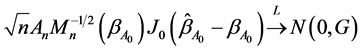
where  is a
is a  matrix such that
 ,
,  is a
is a  non-negative symmetric matrix,
  , and “
 ” represents the convergence in distribution.
Remark: Theorems 1 and 2 imply that the proposed SGEE-QIF procedure is consistent in variable selection, it can identify the zero coefficients with probability tending to 1. By choosing appropriate tuning parameters, the SGEE-QIF estimators have the oracle property; that is, the asymptotic variances for the SGEE-QIF estimators are the same as what we would have if we knew in advance the correct submodel.
3. Computation
3.1. Algorithm
Next, we propose the iterative algorithm to implement the procedures as follows:
Step 1, Calculate the initial estimates  of
of  by solving the initial QIF (2.5) estimator. Let
 .
.
Step 2, By using the current estimate , we choose the tuning parameters
  by the BIC criterion.
Step 3, Update the estimator of  as follows:


where 
and .
.
Step 4, Iterate Steps 2-3 until convergence, and denote the final estimators of  as the SGEE-QIF estimator.
3.2. Choosing the Tuning Parameters
To implement the procedures described above, we need to choose the tuning parameters . Following Ueki [17], we use BIC-type criterion to choose these two parameters. That is, we choose
  as the minimizer of

where  is the SGEE-QIF estimator for given
 ,
,  is simply the number of nonzero coefficient
 . The selected
  minimizes the
 .
.
3.3. Choosing the Basis Matrices
The choice of basis matrices  in (2.2) is not difficult, especially for those special correlation structures which are frequently used. If we assume
  is the first-order autoregressive correlation matrix. The exact inversion
  can be written as a linear combination of three basis matrices, they are
 ,
,  and
and , where
  is the identity matrix,
  has 1 on two main off-diagonals and 0 elsewhere, and
  has 1 on the corners (1, 1) and (m, m), and 0 elsewhere. Suppose
  is an exchangeable working correlation matrix, it has 1 on the diagonal, and
  everywhere off the diagonal. Then
  can be written as a linear combination of two basis matrices,
  is the identity matrix and
  is a matrix with 0 on the diagonal and 1 off the diagonal. More details about choosing the basis matrices can be seen in Zhou and Qu [20].
4. Simulation Studies
In this section we conduct a simulation study to assess the finite sample performance of the proposed procedures. In the simulation study, the performance of estimator  will be assessed by using the average the mean square error (AMSE), defined as
  averaged over
  times simulated data sets.
We simulate data from the model (1.1), where  with
with ,
,  and
and .
.
While the remaining coefficients, corresponding to the irrelevant variables, are given by zeros. In addition, let
 , where
  denotes the largest integer not greater than
 . To perform this simulation, we take the covariates
  from a multivariate normal distribution with mean zero, marginal variance 1 and correlation 0.5. The response variable
  is generated according to the model. And error vector
 , where
  and
and  is a known correlation matrix with parameter
  used to determine the strength of with-subject dependence. Here we consider
  has the firstorder autoregressive (AR-1) or compound symmetry (CS) correlation (i.e. exchangeable correlation) structure with
 . In the following simulations, we make 500 simulation runs and take
  and
and .
.
In the simulation study, for each simulated data set, we compare the estimation accuracy and model selection properties of the SGEE-QIF method, the SCAD-penalized QIF and the Lasso-penalized QIF for two different working correlations. For each of these methods, the average of zero coefficients over the 500 simulated data sets is reported in Tables 1 and 2. Note that “Correct” in tables means the average number of zero regression

Table 1 . Variable selections for the parametric components under different methods when the correlation structure is correctly specified.
Table 2. Variable selections for the parametric components under different methods when the correlation structure is incorrectly specified. The term “CS.AR(1)” means estimation with the fitted misspecified AR(1) correlation structure, while “AR(1).CS” means estimation with the fitted misspecified CS correlation structure.
coefficients that are correctly estimated as zero, and “Incorrect” depicts the average number of non-zero regression coefficients that are erroneously set to zero. At the same time, we also examine the effect of using a misspecified correlation structure in the model, which are also reported in Tables 1 and 2. From Tables 1 and 2, we can make the following observations.
1) For the parametric component, the performances of variable selection procedures become better and better as  increases. For example, the values in the column labeled “Correct” become more and more closer to the true number of zero regression coefficients in the models.
2) Compared with the penalized QIF based on Lasso and SCAD, SGEE-QIF performs satisfactory in terms of variable selection.
3) It is not surprised that the performances of variable selection procedures based on the correct correlation structure work better than based on the incorrect correlation structure. However, we also note that the performance does not significantly depend on working covariance structure.
5. Discussion
In this paper, we have proposed the smooth-threshold generalized estimating equation based on quadratic inference function (SGEE-QIF) to the high-dimensional longitudinal data. Our method incorporates the within subject correlation structure of the longitudinal to automatically eliminate the irrelevant parameters by setting them as zero, and simultaneously estimates the nonzero regression coefficients. As a future research topic, it is interesting to consider the variable selection for the high/ultra-high dimension varying coefficient models with longitudinal data.
Acknowledgements
This research was supported by the National Natural Science Foundation of China (11171012, 11331011), the Science and technology project of the faculty adviser of excellent PHD degree thesis of Beijing (20111000503), the Beijing Municipal Education Commission Foundation (KM201110005029), and the Beijing municipal key disciplines (No.006000541213009).
[2] K. L. Liang and S. L. Zeger, “Longitudinal Data Analysis Using Generalised Estimating Equations,” Biometrika, Vol. 73, No. 1, 1986, pp. 13-22. http://dx.doi.org/10.1093/biomet/73.1.13
[3] A. Qu, B. G. Lindsay and B. Li, “Improving Generalized Estimating Equations Using Quadratic Inference Functions,” Biometrika, Vol. 87, No. 4, 2000, pp. 823-836. http://dx.doi.org/10.1093/biomet/87.4.823
[4] A. Qu and P. X. K. Song, “Assessing Robustness of Generalized Estimating Equations and Quadratic Inference Functions,” Biometrika, Vol. 91, No. 2, 2004, pp. 447-459. http://dx.doi.org/10.1093/biomet/91.2.447
[5] I. E. Frank and J. H. Friedman, “A Statistical View of Some Chemometrics Regression Tools (with Discussion),” Technometrics, Vol. 35, No. 2, 1993, pp. 109-148. http://dx.doi.org/10.1080/00401706.1993.10485033
[6] R. Tibshirani, “Regression Shrinkage and Selection via the LASSO,” Journal of Royal Statistical Society, Series B, Vol. 58, No. 1, 1996, pp. 267-288.
[7] J. Q. Fan and R. Li, “Variable Selection via Nonconcave Penalized Likelihood and Its Oracle Properties,” Journal of American Statistical Association, Vol. 96, No. 456, 2001, pp. 1348-1360. http://dx.doi.org/10.1198/016214501753382273
[8] W. Pan, “Akaike’s Information Criterion in Generalized Estimating Equations,” Biometrics, Vol. 57, No. 1, 2001, pp. 120-125. http://dx.doi.org/10.1111/j.0006-341X.2001.00120.x
[9] H. Akaike, “Information Theory and an Extension of the Maximum Likelihood Principle,” Proceedings of the 2nd International Symposium on Information Theory, Budapest, 1973, pp. 267-281.
[10] L. Wang and A. Qu, “Consistent Model Selection and Data-Driven Smooth Tests for Longitudinal Data in the Estimating Equations Approach,” Journal of the Royal Statistical Society: Series B, Vol. 71, No. 1, 2009, pp. 177-190. http://dx.doi.org/10.1111/j.1467-9868.2008.00679.x
[11] G. Schwarz, “Estimating the Dimension of a Model,” The Annals of Statistics, Vol. 6, No. 2, 1978, pp. 461-464. http://dx.doi.org/10.1214/aos/1176344136
[12] W. J. Fu, “Penalized Estimating Equation,” Biometrics, Vol. 59, No. 1, 2003, pp. 126-132. http://dx.doi.org/10.1111/1541-0420.00015
[13] P. R. Xu, W. Fu and L. X. Zhu, “Shrinkage Estimation Analysis of Correlated Binary Data with a Diverging Number of Parameters,” Science China Mathematics, Vol. 56, No. 2, 2013, pp. 359-377. http://dx.doi.org/10.1007/s11425-012-4564-y
[14] J. Fan and R. Li, “Statistical Challenges with High Dimensionality: Feature Selection in Knowledge Discovery,” Proceedings of the International Congress of Mathematicians, Vol. 3, European Mathematical Society, 2006, pp. 595-622.
[15] J. Fan and J. Lv, “A Selective Overview of Variable Selection in High-Dimensional Feature Space,” Statistica Sinica, Vol. 20, No. 1, 2009, pp. 101-148.
[16] M. Crowder, “On the Use of a Working Correlation Matrix in Using Generalised Linear Models for Repeated Measures,” Biometrika, Vol. 82, No. 2, 1995, pp. 407-410. http://dx.doi.org/10.1093/biomet/82.2.407
[17] L. Hansen, “Large Sample Properties of Generalized Method of Moments Estimators,” Econometrica, Vol. 50, No. 4, 1982, pp. 1029-1054. http://dx.doi.org/10.2307/1912775
[18] M. Ueki, “A Note on Automatic Variable Selection Using Smooth-Threshold Estimating Equations,” Biometrika, Vol. 96, No. 4, 2009, pp. 1005-1011. http://dx.doi.org/10.1093/biomet/asp060
[19] J. Fan and H. Peng, “Nonconcave Penalized Likelihood with a Diverging Number of Parameters,” The Annals of Statistics, Vol. 32, No. 3, 2004, pp. 928-961. http://dx.doi.org/10.1214/009053604000000256
[20] L. Wang, “GEE Analysis of Clustered Binary Data with Diverging Number of Covariates,” The Annals of Statistics, Vol. 39, No. 1, 2011, pp. 389-417. http://dx.doi.org/10.1214/10-AOS846
[21] J. Zhou and A. Qu, “Informative Estimation and Selection of Correlation Structure for Longitudinal Data,” Journal of the American Statistical Association, Vol. 107, No. 498, 2012, pp. 701-710. http://dx.doi.org/10.1080/01621459.2012.682534
[22] J. J. Dziak, “Penalized Quadratic Inference Functions for Variable Selection in Longitudinal Research,” Ph.D Thesis, The Pennsylvania State University, 2006. http://sites.stat.psu.edu/~jdziak/DziakDissert.pdf
Appendix. Proof of Theorems
Proof of Theorem 1
Let . It suffices to prove for any
 , there is a constant
 , such that
 (A.1)
(A.1)
for  enough. This will imply that there exists a local solution to the equation
 . Such that
  with probability at least
 . The proof follows that of Theorem 3.6 in Wang [19], we will evaluate the sign of
  in the ball of
 . Note that
 (A.2)
(A.2)
where  lies between
  and
and  Next we will consider
  and
and  respectively. For
 , by Cauchy-Schwarz inequality, we can derive that

According to condition (C7), consider the  th
th  block of
 ,
,
 , let
, let  denote the
  th components
 , by some elementary calculation, we obtain
where  is the
  th element of
 , hence, we have
 . By C3 and C4, we obtain,
 (A.3)
(A.3)
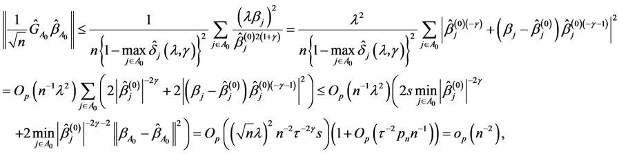
Since , we only need to obtain the convergence rate of
 . Assume that
  is the initial estimator, and is
  -consistent. By using the condition
  for any
  and
and , we have
which implies that  for each
 . Therefore, we have that
 . Hence, by (A.3), we obtain that
 . (A.4)
Now, we consider , we can derive that

By above result, we get . Thus, it is easy to show that for sufficiently large
 ,
,  on the ball of
  is asymptotically dominated in probability by
 , which is positive for the sufficiently large
 . The proof of Theorem 1 is completed.
Proof of Theorem 2
According to Dziak [21], it is known that the initial estimator  obtained by solving the QIF is
  - consistent. For any given
 , by
, by , then,
 (A.5)
(A.5)
which implies that
 (A.6)
(A.6)
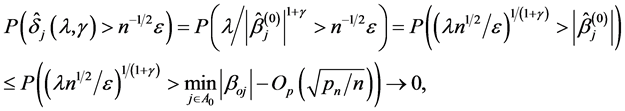
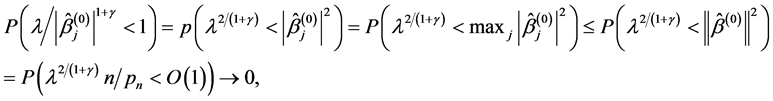
On the other hand, by the condition , for any
 , and
, and , we have

which implies that  for each
 . Therefore, we prove that
 .
.
Thus, we complete the proof of 1).
Next, we will prove 2). As shown in 1),  for
for  with probability tending to 1. At the same time, with probability tending to 1,
  satisfies the smooth threshold generalized estimating equations based on quadratic inference functions (SGEE-QIF)
 (A.7)
(A.7)
Applying a Taylor expansion to (A.7) at , it easy to show that

where . Since, we have
where . Then, if
  holds, by the Slutsky theorem, we can prove Theorem 2 (2). We write
 where
where

Since , we have
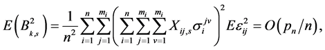
To establish the asymptotic normality, it suffices to check the Lindeberg condition, i.e., for any ,
,
 (A.8)
(A.8)
Using the Cauchy-Schwarz inequality, we have

By Bhebyshev’s inequality,

and
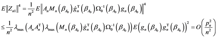
Thus, we have

Therefore,  satisfies the conditions of the Lindeberg-Feller central limit theorem. Hence, the proof of Theorem 2 is completed.