Keywords:Micropolar Fluids; Numerical Analysis; Rotating Disk
1. Introduction
Eringen [1,2] introduced and formulated the theory of micropolar fluids. These fluids exhibit certain microscopic effects due to the local structure and micro motion of the fluid elements. Unsteady flows of micropolar fluid have been considered by a number of authors. Chawla [3] considered the micropolar fluid flow in the neighborhood of a flat plate started impulsively and found the dominant characteristics of two modes of wave propagation during the initial and final stages of growth. Takhar et al. [4] studied the flow of a micropolar fluid past a decelerating porous rotating disk. Lok et al. [5] investigated the boundary layer flow of a micropolar fluid starting impulsively from rest near the forward stagnation point of a plane surface. Guram and Anwar [6] considered the steady, laminar and incompressible flow of a micropolar fluid due to a rotating disk with suction and injection.
The flow of an incompressible viscous fluid past an infinitely rotating disk was first studied by Von Karman [7] who reduced the necessary Navier-Stokes Equations to self-similar form by means of some transformations, and derived approximate solutions. Cochran [8] at a later stage presented accurate numerical solutions to these equations. Another physical solution of importance in this paper is to study the transient state of flow when the disk starts rotating or comes to a halt. Different physical situations were studied in this area by Dolidge [9], Sparrow & Gregg [10] and Benton [11]. Pop [12] investigated the problem of unsteady flow past a wall which starts impulsively to stretch from rest. Sajjad et al. [13] obtained numerical solution for accelerated rotating disk in a viscous fluid. Watson and Wang [14] studied deceleration of a rotating disk in a viscous fluid and found solution of the problem by using fourth order Runge-Kutta algorithm for range . They remarked that similarity solutions do not exist for positive s.
In this paper, we examined the problem of Watson and Wang [14] for micropolar fluids and obtained numerical results for range . The proposed numerical scheme is straight forward, easy to program and very efficient.
2. Mathematical Analysis
The fluid flow is non-steady, laminar and incompressible. The cylindrical coordinates (r, q, z) are used, r being the radial distance from the axis, q the polar angle and z the normal distance from the disk. We assume that there is no body force and body couple. With these assumptions the governing equations of motion for micropolar fluids become:
 , (1)
, (1)
 (2)
(2)
 . (3)
. (3)
By using the following similarity transformations:
 (4)
(4)
where  is the dimensionless variable, n being kinematics viscosity,
  is constant and
 is a positive constant, the velocity is
  and micro rotation is
 . When
 , the problem reduces to the case of the steady rotation of a disk in a fluid. We shall study the case when
 . The equation of continuity (1) is identically satisfied and Equations (2) to (3) yield:
 , (5)
, (5)
 , (6)
, (6)
 , (7)
, (7)
 , (8)
, (8)
 , (9)
, (9)
 , (10)
where primes denote differentiation with respect to  and
and . The material constants
 ,
,  ,
,  and
and
 all are non-dimensional and are given by

The boundary conditions are:
 (11)
(11)
The governing third order ordinary differential equations are reduced to second order ODE’s.
let  (12)
(12)
Then, Equations (5)-(9) become
 , (13)
 , (14)
 , (15)
 , (16)
 . (17)
The boundary conditions (11) become
 (18)
(18)
In order to obtain the numerical solution of nonlinear ordinary differential Equations (13) to (17), these equations are approximated by central difference approximation at a typical point  of the interval [0,¥) and then solved by using SOR method. The first order ordinary differential equation (12) is solved by Simpson’s (1/3) rule with the formula given in Milne [15]. Higher order accuracy O(h6) is achieved, on the basis of above solutions by using Richardson’s extrapolation.
3. Numerical Results and Discussion
The numerical results have been computed for three different grid sizes namely h = 0.5, 0.025, 0.0125 for the comparison purpose. The results are obtained for several values of the parameter s in the range  and for three different sets of the material constants
  and
and  given below:
The numerical results of the velocity components namely f the axial component, g the circumferential component and  the radial component along with the microrotation components L, M, N are given in Tables 1 to 3 in the case-I. The results for f are computed by Simpson’s (1/3) rule and the results for f,
  , g, L, M and N have been computed by SOR method and presented in these tables on finer grid size. The results of velocity components, using Richardson extrapolation are given in the Tables 4 to 5 for some representative values of s.
Graphically, the results have also been demonstrated. Figure 1 represents the behavior of f. It is observed that  decreases for increasing the magnitude of s. Figure 2 depicts
 . Figure 3 exhibits
  which also decreases in magnitude with increase in magnitude of s. Figures 4 and 5 show the microrotation components L and M.

Table 1. s = 0.2.
Table 2. s = 1.0.
Table 3. s = 2.0.
Table 4. s = 2.0.
Table 5. s = 3.0.
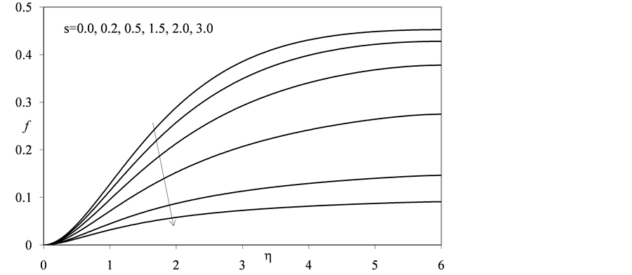
Figure 1. Graph of f for different values of s.

Figure 2. Graph of g for different values of s.

Figure 3. Graph of  for different values of s.

Figure 4. Graph of L for different values of s.

Figure 5. Graph of M for different values of s.
4. Conclusion
The unsteady flow of micropolar fluids about an accelerated rotating disk is discussed in detail. The set of difficult non-linear ODE’s is solved by using a very easy and efficient numerical scheme. The accuracy of the results is checked by comparing the results for three different grid sizes. The constants “C’s” affect the micro rotation of micropolar fluids flow. If one of these constants  is close to zero the micropolar fluid flow resembles the Newtonian fluid flow. It is noted that velocity and microrotation components decrease in magnitude as the parameter s increases in value.
NOTES
*Corresponding author.