Discrete Singular Convolution Method for Numerical Solutions of Fifth Order Korteweg-De Vries Equations ()
1. Introduction
The study of travelling wave solutions of nonlinear partial differential equations (PDEs) is the major subject in many fields of physical and nonlinear sciences. Concepts like solitons, peakons, kinks, breathers, cusps and compactons have entered into various branches of natural sciences such as chemistry, biology, mathematics, communication and particularly in almost all branches of physics like the fluid dynamics, plasma physics, field theory, nonlinear optics and condensed matter physics. Among these nonlinear PDEs there exists an important class of the fifth order Korteweg-de Vries equations
 (1)
(1)
where 
 ,
,  and
and  are real numbers. This class includes the well-known Lax [1], Sawada-Kotera (SK) [2], Kaup-Kupershmidt (KK) [3] and Ito [4] equations. The knowledge of close form solutions of nonlinear PDEs facilitates the verification of numerical solvers, aids physicists to better understand the mechanism that governs the physic models, provides knowledge to the physical problem, provides possible applications and helps mathematicians in the stability analysis of solutions. While strange attractors and chaos theory give us a better understanding of the erratic and often unpredictable nature of natural phenomena, and soliton theory helps explain natural phenomena that are surprisingly predictable and regular even under conditions that would normally destroy such properties. A soliton is a solitary wave which preserves its shape and velocity after nonlinearly interacting with other solitary waves or (arbitrary) localized disturbances.
In general, Equation (1) does not admit exact solutions, therefore one has to resort to numerical methods. Due to the fifth-order terms in these equations, it is very difficult to compute the solutions of these equations accurately and efficiently. Recently, Shen [5] proposed a new dualPetrov-Galerkin method for the third and higher oddorder equations. His approach was proven to be very effective for the KdV type equations in bounded domains [5] and in semi-infinite intervals [6]. In [7], a numerical scheme based on the dual-Petrov-Galerkin method was proposed and implemented for the Kawahara and modified Kawahara equations.
In this paper, we propose a discrete singular convolution method to solve fifth order Korteweg-de Vries equations. Discrete singular convolution (DSC) methods belong to the family of local spectral (LS) methods. They were proposed by Wei [8] as a potential approach for numerical realization of the Hilbert transform, Abel transform, Random transform and Delta transform. The DSC algorithm has been essential to many practical applications, such as nonlinear equations [9], structural analysis [10,11], compressible and incompressible fluid flows [12,13], electromagnetic wave propagation, scattering [14, 15] and image analysis [16].
Recently, Pindza and Maré [17] utilized a combined fourth order exponential time differencing of Adams type and the DSC method to solve the generalized Kortewegde Vries. Their approach revealed exponential convergence. The advantage of the DSC methods is that they exhibit exponential convergence of spectral methods [18] while having the flexibility of local methods for complex boundary conditions [10,19].
The discretization of the generalized Korteweg-de Vries equations in space with the DSC method yields a system of ordinary differential equations (ODE) that needs to be solved by time integration methods. We use the fourth order exponential time differencing Runge Kutta (ETDRK4) [20] for the solution of the resulting semidiscrete equations. The matrix exponential required by the scheme is efficiently computed using best rational approximations based on the Carathéodory-Fejér (CF) procedure [21].
The layout of this paper is as follows. We describe the formulation of the DSC method in Section 2. In Section 3, we discuss the exponential time integration methods for solving the semi-discrete system resulting from the spatial discretization of the nonlinear PDEs. Numerical results illustrating the merits of the new scheme are given in Section 4 and we present our conclusions in Section 5.
2. Discrete Singular Convolution Methods
Discrete singular convolution (DSC) methods are relatively new numerical techniques in the field of nonlinear equations. They are defined as follow. Consider a distribution,  and
and  an element of the space of test functions. A singular convolution can be defined by
 (2)
(2)
where  is a singular kernel. For many science and engineering problems, an appropriate choice of
  has to be done. For instance, in the field of interpolation of surfaces and curves the singular kernel of delta type
  is very important. For numerical solutions of partial differential equations, the kernel
  is essential, where the subscript n denotes the
  -th order derivative of the distribution with respect to parameter
 . While using the DSC method, numerical approximations of a function and its derivatives can be treated as convolutions with some kernels. According to the DSC method, the
  -th derivative of a function
  can be approximated as [22]
 (3)
(3)
where  is the grid spacing,
  is the set of discrete grid points which are centered around
 , and
, and  is the effective kernel, or computational bandwidth; and is usually smaller than the whole computational domain.
In the present paper, we focus our attention on the regularized Shannon kernel (RSK)
 (4)
(4)
to provide discrete approximations to the singular convolution kernels of the delta type (3). The required derivatives of the DSC kernels can be easily obtained using ([12])
 (5)
(5)
The error estimation of the regularized Shannon kernel (RSK) delivers very small truncation errors when it uses the above convolution algorithm ([23])
Theorem 2.1 (Qian [23]). Let  be a function and band limited to
 ,
,
 Then
Then
 (6)
(6)
where  and
and 
Here  is the number of grid points. The
  error given by (6) decays exponentially with respect to the increase of the DSC band width
The proof of the above theorem is beyond the scope of this paper. We refer the reader to [23] for a detailed discussion on the Shannon’s sampling theorem.
Using (4) and (5), the entries of the first, second, third and fifth differentiation matrices ,
,  ,
,  and
and  are given explicitly by
 (7)
(7)
 (8)
(8)
 (9)
(9)
 (10)
(10)
Note that the differentiation matrix in (5) is in general banded. This gives rise to great advantage in large scale computations. Extension to higher dimensions can be realized by tensor products.
The choice of ,
,  and
and  was suggested by Qian and Wei [23]. For instance, if the
  norm error is set to
  the following relations must be satisfied
 (11)
(11)
where  and
and  is the frequency bound of the underlying function
 .
.
To illustrate the procedure of discretization of PDEs by the DSC method, we consider the computation of fifth order KdV equations given by
 (12)
(12)
where ,
,  ,
,  and
and  are real numbers and
 .
.
This equation was previously considered in [24] where its properties were studied and its analytical soliton solutions were revealed. In the present paper we mainly focus on numerical solutions of Equation (12) via the use of DSC method.
The semi-discretized version, at the  th row, of the equation in consideration is obtained by substituting the relations (3) and (5) into (12), yielding
 (13)
(13)
where ,
,  ,
,  and
and  are the typical elements of matrices
 ,
,  ,
,  and
and , respectively. Therefore, Equation (13) can be expressed in the following matrix form
 (14)
(14)
where  represents the linear part of the system and
represents the nonlinear part.
The main difficulty when dealing with systems of the type (14) is that the use of explicit time integrators is inefficient because the system typically suffers from instability due to the higher order derivative. This was emphasized by Pindza [25]. Consequently, the time step size must be significantly reduced in order to fulfill the drastic stability condition present in explicit time integrators. In this paper we use the fourth order exponential time differencing Runge-Kutta method.
3. Exponential Time Differencing
Exponential time differencing (ETD) schemes are known for a long time in computational electrodynamics; see [26] for a comprehensive review of ETD methods and their history. In this section, we describe the exponential time differencing fourth-order Runge-Kutta (ETD4RK) method which was proposed by Cox-Matthews [27].
The main idea of the ETD methods is to multiply both sides of a differential equation by some integrating factor, then we make a change of variable that allows us to solve the linear part exactly and, finally, we use a numerical method of our choice to solve the transformed nonlinear part.
3.1. Overview of the Method
In order to elaborate on this approach, let us consider the following semi-linear partial differential equation
 (15)
(15)
where  and
and  are the linear and nonlinear operators, respectively. The semi-linear partial differential equation is discretized in space with the discrete singular convolution method. Therefore, we obtain a system of ordinary differential equations (ODEs)
 (16)
(16)
The exponential time differencing (ETD) methods can be obtained by integrating Equation (16) exactly between the time steps  and
and  with respect to
 , to obtain
 (17)
(17)
There exist various ETD methods for the evaluation of (17). The purpose of this work is not to give a complete classification of ETD methods. We focus specifically on the fourth order exponential time differencing RungeKutta (ETDRK4) given by
 (18)
(18)
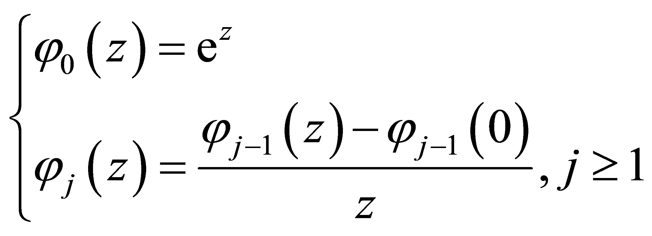
The main computational challenge in the implementation of exponential time differencing (ETD) methods is the need for fast and stable evaluations of exponential and related  -functions
 (19)
(19)
i.e., functions of the form . The computation of these functions depends significantly on the structure and the range of eigenvalues of the linear operator and the dimensionality of the semi-discretized PDE. Unfortunately, for DSC methods the linear part have eigenvalues approaching zero, which leads to complications in the computation of the coefficients. Saad [28], and Hochbruck and Lubich [29] introduced Kyrlov methods to compute
  -functions. Kassam and Trefethen [20] used Cauchy integral representation on a circle for a stable computation of
  -functions. Our evaluation of exponential and related
  -matrix functions follows the idea of Schmelzer and Trefethen [30]. This method is based on computing optimal rational approximations to the matrix functions on the negative real axis using the Carathéodory-Fejér (CF) procedure [21], closely. The
  - functions (19) can be computed explicitly by a recursive formula
 (20)
(20)
Another way to compute the functions  is to use the Taylor series representation. Therefore, for all complex numbers
 , we have
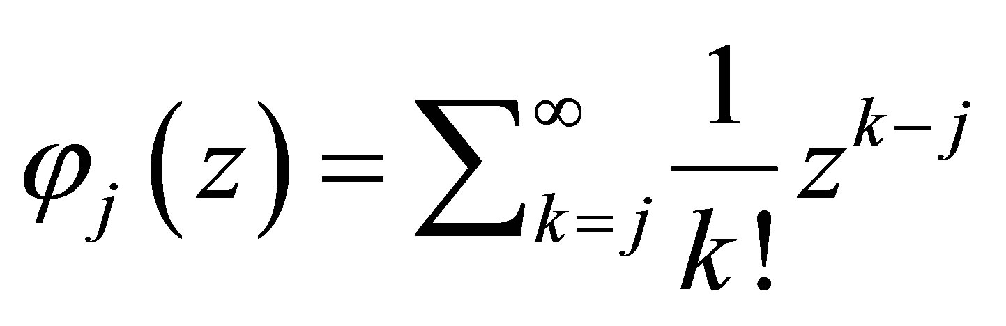 (21)
(21)
However, it is known that the computation of these functions in their explicit or Taylor series form suffers from computational inaccuracy for matrices whose eigenvalues are equal to or approaching zero. This is generally the case when the spatial discretization is based on spectral methods. In order to overcome the numerical difficulties encountered in the computation of (20) and (21), a different tactic for evaluating the function was proposed in [20]. The key idea is to approximate the functions (for matrices or scalars) by means of contour integrals in the complex plane
 (22)
(22)
where . If the contour
  encloses the spectrum of the non-diagonal matrix
  we have
 (23)
(23)
If the size of the matrix  is large, it is more advantageous to compute the product of the functions
  and vectors
  rather than to compute
  explicitly. We have
 (24)
(24)
where  and
and  are the poles and the residues, respectively. The sum in (24) is evaluated by solving at most
  shifted linear systems. The poles and the residues are computed efficiently in standard precision by the Carathéodory-Fejér method [21,30].
3.2. Stability Analysis
In this section, we investigate the linear stability of the ETDRK4 method for the nonlinear autonomous system of ODEs,
 (25)
(25)
linearized about a fixed point  such that
  We obtain
 (26)
(26)
where u is now the perturbation of  and
and 
is a diagonal or a block diagonal matrix containing the eigenvalues of . If
. If , then the fixed point
  is stable for all
 .
.
The stability region is four-dimensional, if both  and
and  are complex. The two-dimensional stability region is obtained if both
  and
and  are purely imaginary or purely real, or if
  is complex and
  is fixed and real.
In the paper, we follow the analysis employed in [27] and we only concentrate on the case where  and
and  are real. We define
 ,
,  and
and . Then, applying the ETDRK4 method (18) to the linearized problem (26) yields
 (27)
(27)
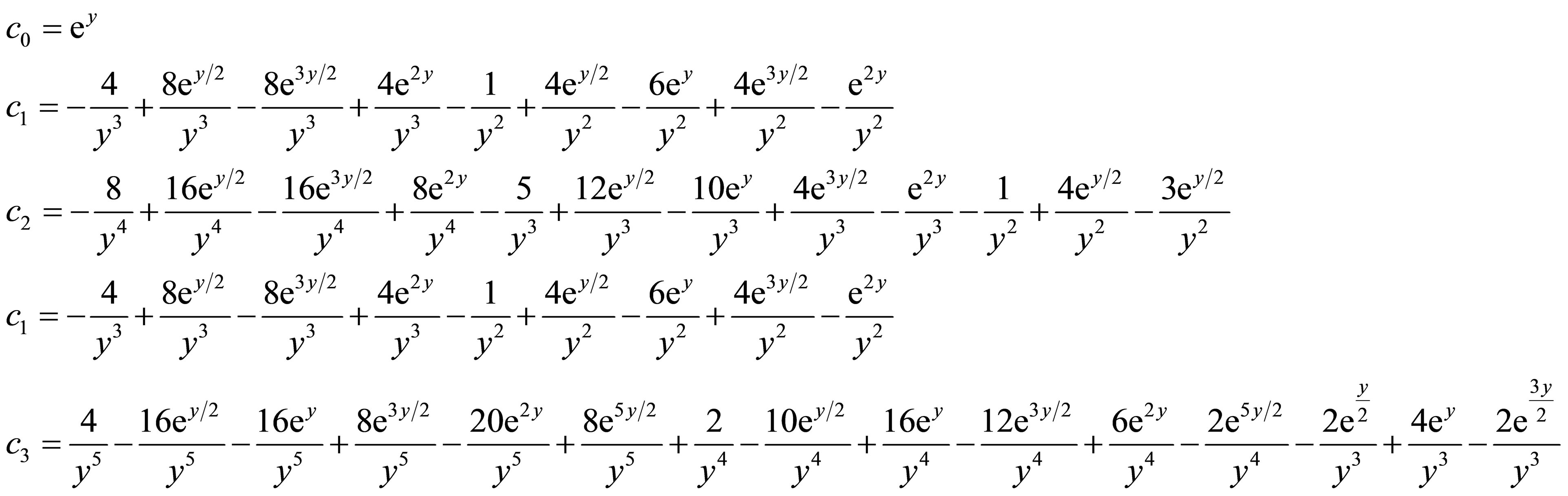
However, one can observe that the computation of ,
,  ,
, and
and  suffers from computational inaccuracy for values of
  equal to or approaching zero. Therefore, it is important to make use of their Taylor expansions

We commence our analysis by choosing real negative values of  and looking for a region of stability in the complex
  plane where
 . Hence, the boundary of the stability region is determined by writing
The corresponding families of stability regions are plotted in the complex  plane and displayed in Figure 1. Note that, in this figure, the horizontal and the vertical axes represent
  and
and , respectively. Clearly, as shown in Figure 1, the stability region for the ETDRK4 scheme grows larger as
 . The red curve corresponds to the case
 , where the stability region of the ETDRK4 scheme coincides with that of the corresponding order fourth order Runge-Kutta (RK4) scheme.
4. Numerical Results
method for solving the fifth order KdV equation. To show the efficiency of the present method, we report the relative infinity and root mean square norm errors of the solution defined by
 (28)
(28)
and
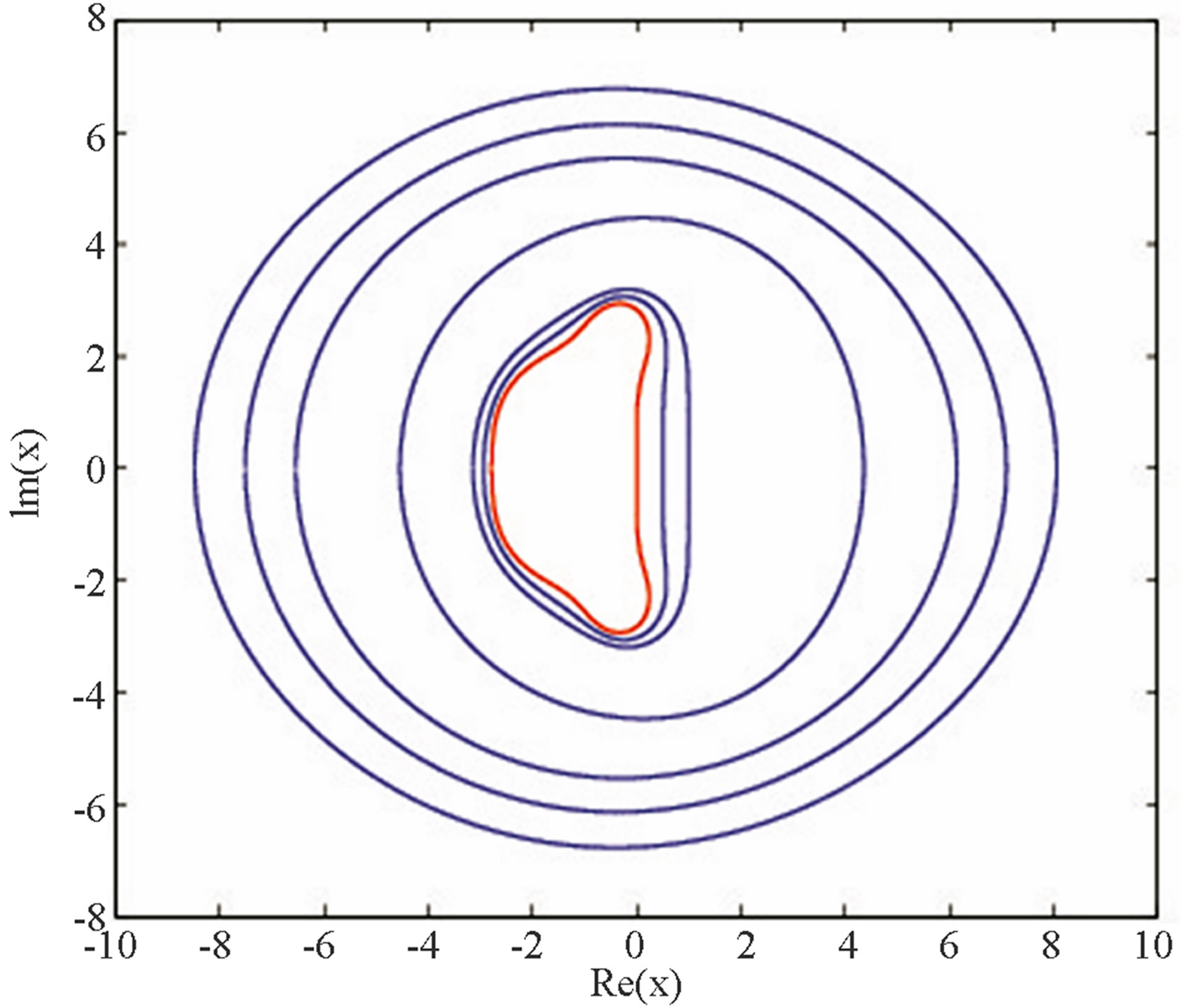
Figure 1. Stability regions in the complex x plane. The curves correspond to , from the outer curve to the inner curve respectively. The inner red curve corresponds to y = 0.
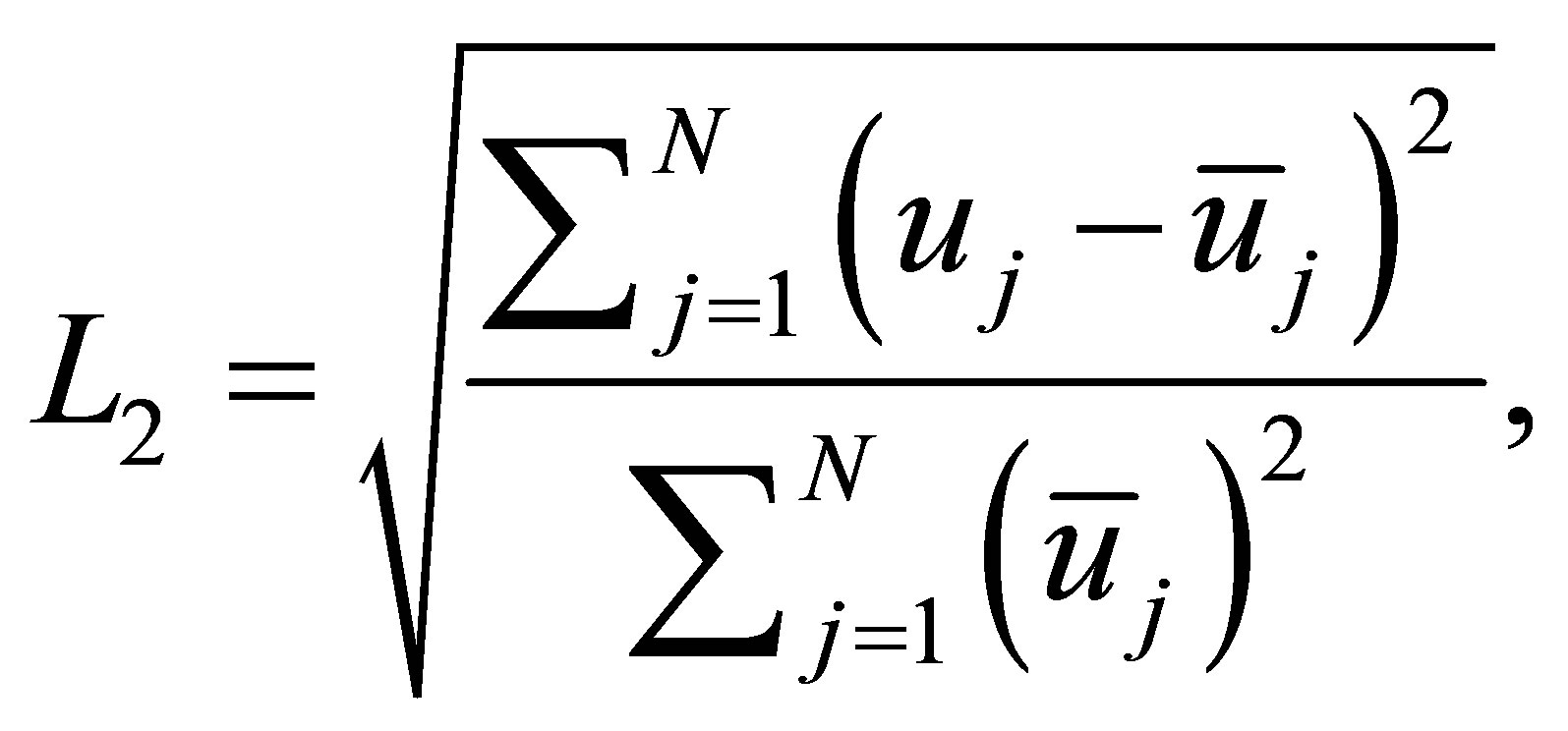 (29)
(29)
respectively, where  is the number of interior points,
  and
and  are the exact and computed values of the solution
  at point
 .
.
In this paper, we consider two case studies depending on the set of parameters of (25) that provide multi-soliton solutions. We evaluate the performance the DSC algorithms for different time increment , spatial discretization
 , the support size of DSC kernels
  and regularization parameter
 .
.
In our computation, the first set of parameters that we select are given by . In this case, the fifth order KdV Equation (11) is known as the SawadaKotera (SK) [2] equation and is given by
 (30)
(30)
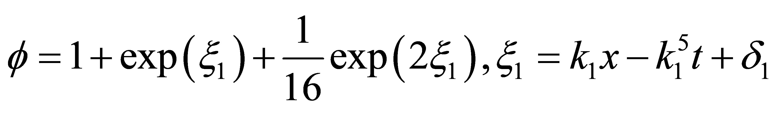
The SK (30) admits multi-soliton solutions [31]. The derivation of these soliton solutions is beyond the scope of this paper. We only list them here for testing numerical procedures purposes. Single and two soliton solutions are given by
 (31)
(31)
where
 (32)
(32)
 (33)
(33)
respectively, with
 (34)
(34)
In our computational work, we use the collocation points
 (35)
(35)
The SK equation possesses infinite conservation laws [31]. The first three conservation laws are given as follow
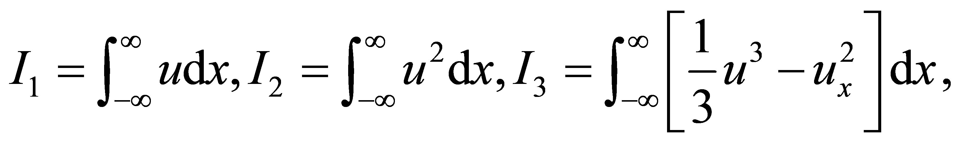 (36)
(36)
related to the mass, momentum and energy. The quantities ,
,  and
and  are applied to measure the conservation properties of the collocation scheme, calculated by
 (37)
(37)
The second set of parameters are chosen as  . This is well-known as the KaupKupershmidt (KK) [3] equation
 (38)
(38)
Multi-soliton solutions can be generated by the following nonlinear transformation of the dependent variable,
 (39)
(39)
For one soliton solution, the dependent variable function is given by
 (40)
(40)
For two soliton solutions, the dependent variable function is
 (41)
(41)
with
 (42)
(42)
The KK equation possesses infinite conservation laws [31], the first three are given as follows
 (43)
(43)
The quantities ,
,  and
and  are applied to measure the conservation properties of the collocation scheme, calculated by
 (44)
(44)
In next sections, we study the propagation and the interaction of single and two soliton solutions, respectively.
4.1. Propagation of Single Solitons
In our numerical experiments, we first model the motion of a single soliton of the SK (30) and KK (38) equations. For the SK equation, the initial condition is taken from the exact solutions (32) and (31) at initial profile. Whereas for the KK equation, the initial condition is taken from the exact solutions (40) and (39) at initial profile. The boundary conditions in both cases are chosen so that
 (45)
(45)
In the first computation, we would like to investigate the convergence of the DSC method with respect to the number of grid points  and the DSC bandwidth
 . The values of the parameters used in our numerical experiments are:
  and
and  in both cases of the SK and KK equations. In each case, the soliton moves to the right across the space interval
  when the time interval is
 . The choice of the DSC bandwidth
  and the regularizer parameter
  is done according to the conditions (10). Hence if
  then
then . If
. If  then
then . If
. If  then
then .
.
Figure 2 illustrates the convergence of the DSC with respect to the number of the grid points  and the DSC bandwidth
 . We observe that numerical soliton solutions of the DSC method converge towards the exact soliton solutions as the number of grid points
  increases. We remark that the convergence of the DSC method also relies on the bandwidth
 . The results in Figure 2 shows that the case
  gives a better convergence, the case
  gives the worst convergence, whereas when
  we have an intermediate convergence.