Application of Improved Analysis of Variance to Ionospheric TEC Short-Term Forecast ()
1. Introduction
In order to improve the performance of radio systems, such as communication system, positioning system, radar, navigation et al, and to ensure the safety of space flight, much more precise forecast of ionosphere is becoming indispensable. Short-term forecast which predicts the ionosphere weather change in time scale of days or hours is the development trend [1]. Currently, short-term ionospheric forecast is mainly carried out in America, Europe and Australia et al. with various methods including autocorrelation analysis [2,3], multiple linear regression method [4,5], artificial neural network method [6], the storm-time ionospheric empirical correction model [7,8], interpolation of regional ionospheric forecast [9], equivalent sunspot number method [10,11], ionospheric assimilation model [12,13] et al. Different methods are used in different countries as the ionosphere is different from region to region. So it is necessary to build our own model for short-term forecast of ionosphere which is suited to China.
In China, ionospheric modeling and forecasting plays a key role in this study field. And many models and methods such as Asia region ionospheric F2 layer prediction method [15], Chinese reference ionosphere [16], middle and low latitude F layer power Numerical simulation of characteristics [17], characteristics of ionospheric region [18] and other methods are developed. But most of them are only capable of long-term forecast rather than short-term. Although some research has been done in short-term forecasting modeling, a practical approach hasn’t been achieved so far.
Variance analysis has been studied in this paper, an improved method based on superposition analysis of periodical wave variance has been applied to short-term forecast of ionosperic TEC (Total Electron Content). The forecasting precision of this method was analyzed quantitatively before and after it’s improved with reference ionospheric TEC data provided by IGS (International GNSS Service).
2. Improved Superposition Analysis of Periodical Wave Variance
Superposition analysis of periodical wave variance is a pure statistical forecast method. The basic principle is to analyze the period of a certain length of processed historical data, and superpose different periods of data together to fit with the historical data, and then extrapolate to make quantitative prediction of the future [19] Ionospheric TEC data was recorded at a particular time with a fixed time interval so can be analyzed as time series.
2.1. Superposition Analysis of Periodical Wave Variance
Superposition analysis of periodical wave variance for time series analysis should make time series data arranged with assumption period, if variance within the group is less than that between the groups, the arranged period matches to the actual, then the forecasting could be performed. It takes the following three steps to make a prediction.
1) The first cycle analysis.
With time series , assuming there is a periodic vibration of length of
 , the elements are arranged in
  period. If the remaining elements are less than
 , they will be arranged at the bottom line. Each column is a group and the sums of deviation squares are calculated respectively within and among groups, which are respectively caused by the random error and the difference of mean values of each group. The variance is divided by the respective freedom to obtain the mean square deviation to structure the corresponding
  statistics.
The maximum value of  is selected as test period to compare with
  which could be checked in the
 test critical table. When (if)
 , there is significant difference in the group. After the first cycle measured, the corresponding mean value of each column is as the first cycle component, which could construct a periodic sequence by arranging the mean values in corresponding order.
2) The further cycle analysis.
Remaining series which are the residuals can be obtained by subtracting the first cycle component from the original value. And it needs to be analyzed again with the approach described above. But if , a third cycle analysis needs to be done. Follow-up cycles are detected until
 , which means that there is no significant cycle any more.
3) Return test and forecast.
Periodic components would be superposed to obtain the return value of the original series and prediction value could be obtained by extrapolation.
2.2. Forecasting Model Building and Improving
In superposition analysis of periodical wave variance, elements of each column minus the corresponding mean value to get the corresponding periodic component after period is detected, which shows all the epoch's contribution is consistent (all the epoch contributes the same) in extrapolation forecast. However, the changes of the ionosphere TEC are not always smooth, which perform increase and decrease, so the contribution about different epochs in the forecast is not same. In order to improve forecasting precision further, each column of the original data is weighted and then the corresponding periodic component is obtained by the weighted values.
To select a certain length of the ionospheric TEC historical data and obtain periodic components by variance analysis, then superimpose periodic components together. When the fitting precision to historical data meets the required level, the quantitative prediction of the trend could be obtained by extrapolation.
Short-term forecasting model of the ionospheric TEC models is as follows:
1) The first cycle analysis.
Suppose there is ionospheric TEC time series:
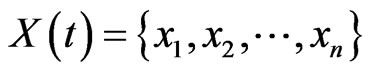
where, n is the number of epochs. Taking
 , the TEC raw data are arranged in the cycle of T and each row is a T cycle:
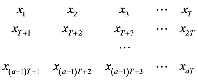
where, . If
. If ,
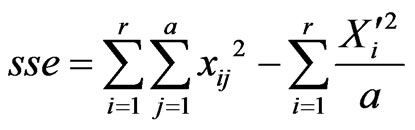
,  are arranged at the bottom line. Each column is a group and the sums of deviation squares are calculated respectively within and among groups:
 (1)
(1)
 (2)
(2)
where, a is the number of columns, r is the number of rows and  is the sum of each row. The sums of deviation squares are represented sse and ssa respectively within and among groups.
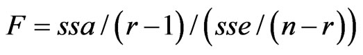
Since ionospheric TEC data are independent, sse and ssa obey the distribution of  and F statistics constructed:
 (3)
(3)
where, r-1 and n-r are the freedom degrees.
The weighted value:
 (4)
(4)
The first cycle can get by making the comparison between the max  value and
  which can be checked in the
  test critical table. The corresponding weighted value of each column is used as the first cycle component, which forms a periodic series by arranging in order. Remaining series could be obtained through the raw series minus the first cycle component.
2) The follow-up cycle analysis.
Remaining series are used as new time series to continue variance analysis by repeating steps 1, 2 until no significant cycle.
3) Return to the raw data test and make prediction of ionospheric TEC.
Superimposing all components of significant periods mentioned above, the test value in return of raw data could be obtained and also the quantitative prediction of future trend by extrapolation.
3. Examples and Results
In this paper, the precision of the method improved or not is analyzed through calculating ionospheric TEC data in 2008 provided by IGS, which is selected randomly. Then the calculation of 40 days is taken as the example for analysis. Since the sampling rate of the IGS TEC data is , data calculated with superposition analysis of periodical wave variance including improved and unimproved is selected (N30°, E105°), (N35°, E105°), (N40°, E105°), (N30°, E100°), ( N30°, E95°), (N30°, E90°) and (N30°, E85°) from Jan. 11 to Feb. 19 to obtain the prediction of ionospheric TEC about this region in Feb. 20 and Feb. 21 in 2008 by superimposing the cycle components. The calculation about (N30°, E105°) from Jan. 11 to Feb. 19 in 2008 is taken as the example for analysis. Figure 1 shows the results.
This method has an average fitting precision about 0.8 TECU according to multiple experiments, 0.5 TECU is the best. But about 10% of all the epochs have relatively large error. These epochs are from Beijing Time (BT) 2:00 to 8:00 everyday, which indicates that the improved method has a better performance from 9:00 (BT) to midnight. Obviously in Figure 2, TEC changes regularly from 5:00 to 8:00, irregularly form 8:00 to 12:00 which happen to be 0:00 (BT) to 8:00 (BT). This cannot be just a coincidence, the bad forecasting precision during this
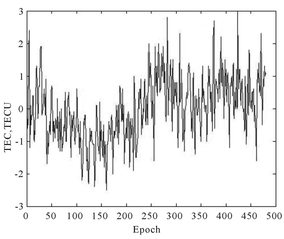
Figure 1. Residual error distribution of observation and pay-back checking value from Jan. 11 to Feb. 19 in 2008.
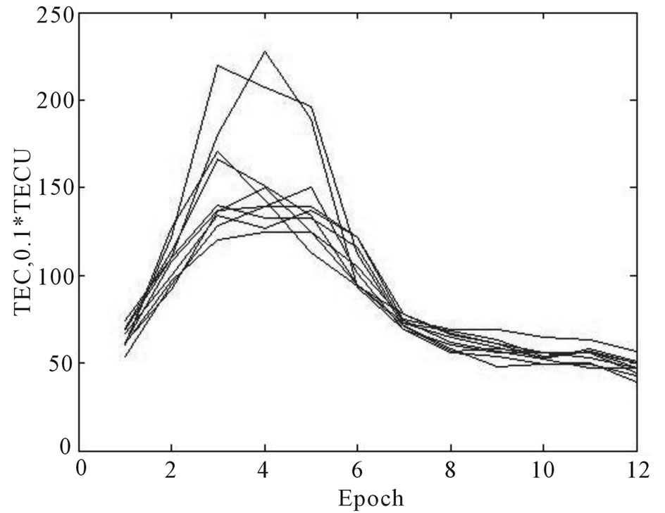
Figure 2. The TEC variation from Jan. 11 to Jan. 20 in 2008.
time period must has something to do with the irregular change of ionosphere. And in this study, it’s the main cause of the bad fitting.
A lot of extrapolation experiments have been conducted and here (N40°, E105°), (N35°, E105°) and (N30°, E105°) are chosen as examples to show the results. We plot residuals (the forecasted value subtracted the real value from IGS) of these three locations respectively with the original method and the improved method as well (as is shown in Figures 3-5). Clearly, almost all the absolute values of the residuals are no more than 3 TECU except several epochs at N30. And the precision is much better when using the improved method. Wang from Xian University of Electronic Science and Technology gave a prediction precision of 0.75-3.75 TECU in his master thesis by using auto-correlation method. Using the improved method the RMS are 1.537 TECU, 1.258 TECU, 2.292 TECU at the three locations respectively which means this method has good forecasting precision.
TEC data at (N30°, E100°), (N30°, E95°), (N30°, E90°) and (N30°, E85°) has been selected for variance analyzing and extrapolation forecast to explore the relationship between geographical longitude and the forecasting precision of this method, the RMS is shown in Figure 6.
Figure 6 indicates that the forecasting precision is related to longitude and latitude, especially latitude. In the northern hemisphere, the RMS is proportional to longitude and inversely proportional to latitude, which means the precision will decrease in regions with higher longitudes and lower latitudes, and these places are happen to be with intensely changed ionosphere. In addition, Figure 4 shows that the forecasting precision isn’t very good at noon in China when the ionosphere changes very severe. Therefore, future studies should focus on how to improve the prediction precision when ionosphere changes intensely.