1. Introduction
A graph invariant is any function on a graph that does not depend on a labeling of its vertices. Topological indices and graph invariants based on the distances between the vertices of a graph are widely used in theoretical chemistry to establish relations between the structures and the properties of molecules. Topological indices provide correlations with physical, chemical and thermodynamic parameters of chemical compounds [2]. In this paper, we only consider simple and connected graphs. Let G be a graph on n vertices and  edges. We denote the vertex and the edge set of G by
  and
and , respectively. As usual, the distance between the vertices
  and
and  of G, denoted by
  (
( for short), is defined as the length of a minimum path connecting them. We let
  be the degree of a vertex
  in G. The eccentricity, denoted by
 , is defined as the maximum distance from vertex
  to any other vertex. The diameter of a graph G, denoted by
 , is the maximum eccentricity over all vertices in a graph G.
The Cartesian product  of graphs G and H is a graph such that
 , and any two vertices
  and
and  are adjacent in
  if and only if either
  and
and  is adjacent to
 , or
, or  and
and  is adjacent to
 , see [3] for details. Let
  and
and  be two graphs with disjoint vertex sets
  and
and  and edge sets
  and
and . The join
  is the graph union
  together with all the edges joining
  and
and . The composition
  is the graph with vertex set
  and
and  is adjacent to
  whenever (
 is adjacent with
 ) or (
 and
and  is adjacent to
 ), [3, p. 185]. The disjunction
  of graphs
  and
and  is the graph with vertex set
  and
and  is adjacent to
  whenever
  or
or . The symmetric difference
  of two graphs
  and
and  is the graph with vertex set
  and
and
 .
.
The first Zagreb index was originally defined as
 [4]. The first Zagreb index can be also expressed as a sum over edges of
 ,
,
 We refer readers to [5]
for the proof of this fact and for more information on Zagreb index. The first Zagreb coindex of a graph  is defined in [6] as:

Let  be the number of pairs of vertices of a graph
  that are at distance
 ,
,  be a real numberand
 , that is called the Wienertype invariant of
  associated to
 , see [7,8] for details. Additively weighted Harary index is defined in [9] as

Dobrynin and Kochetova in [10] and Gutman in [11] introduced a new graph invariant with the name degree distance that is defined as follows:

In [12], the modified degree distance was defined as follows:

The generalized degree distance, denoted by , is defined as follows in [1].
For every vertex  and real number
 ,
,  is defined by
 , where
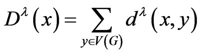 . We then define

If , then
 . When
 , this new topological index
  is equal to the degree distance (or Schultz index). There are many papers for studying this topological index, for example see [13-16]. Also if
 , then
  Therefore the study of this new topological index is important and we try to obtain some new results related to this topological index. The modified generalized degree distance, denoted by
 , is defined in [1] as:
If , then
 .
.
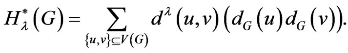
We construct graph polynomials having the property such that their first derivatives at  are equal to the generalized degree distance, the modified generalized degree distance and Wiener-type invariant respectively. These polynomials are defined as follows:

and

The Wiener index of the Cartesian product of graphs was studied in [17,18]. In [19], Klavžar, Rajapakse and Gutman computed the Szeged index of the Cartesian product of graphs. In [9,20-24], exact formulae for the hyper-Wiener, the first Zagreb index, the second Zagreb index and Schultz polynomials of some graph operations were computed.
Throughout this paper,  and
and  denote the cycle, path, complete graph and star on
  vertices. The complement of a graph
  is a graph
  on the same vertices such that two vertices of
  are adjacent if and only if they are not adjacent in
 . The graph
  is usually denoted by
 . Our other notations are standard and taken mainly from [2,25,26].
In this paper we present explicit formulas for  of graph operations containing the Cartesian product, composition, join, disjunction and symmetric difference of graphs and introduce generalized and modified generalized degree distance polynomials of graphs, such that their first derivatives at
  are respectively, equal to the generalized degree distance and the modified generalized degree distance. These polynomials are related with Wiener-type invariant polynomial of graphs.
2. Main Results
The aim of this section is to compute the generalized degree distance for five graph operations. We start with a lemma which gives some information about the number of vertices and edges of operations on two arbitrary graphs. For a given graph , the number of vertices and edges will be denoted by
  and
and , respectively.
Lemma 2.1. [3,20] Let  and
and  be graphs. Then we have:
a)

and

b) The graph  is connected if and only if
  and
and  are connected.
c) If  and
and  are vertices of
 , then
 .
.
d) The Cartesian product, join, composition, disjunction and symmetric difference of graphs are associative and all of them are commutative except the composition of graphs.
e)
 .
.
f)

g)
h)

i) 
j) 
k) 
l)

m)

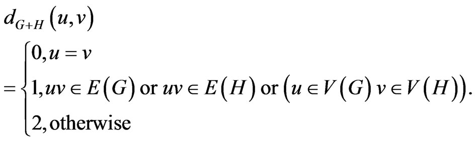
In Theorem 2.2, we give a formula for the generalized degree distance of the join of two graphs.
Theorem 2.2. Let  and
and  be two graphs. Then
Proof. It is obvious from definition that for any , the distance
  is either 1 or 2. In the formula for
 , we partition the set of pairs of vertices of
  into three subsets
  and
and . In
. In  we collect all pairs of vertices u and v such that u is in
  and v is in
 . Hence, they are adjacent in
 . The set
  is the set of pairs of vertices u and v which are in
 . Also we partition the sum in the formula of
  into three sums
  so that
  is over
  for
for . For
. For  we obtain

and

Similarly,

Therefore
 □
□
Corollary 2.3. Let G be a connected graph with n vertices and m edges. Then
 .
.
The exact formulas  for the fan graph K1 + Pn and for the wheel graph
  are given in the following Corollary.
Corollary 2.4.

and

Remark 2.5. In the above theorem, if , then we obtain
 , which gives first derivatives formula Theorem 3 in [22] at
 .
.
In the next theorem we obtain the exact formula for the generalized degree distance of the composition of two graphs.
Theorem 2.6. Let  and
and  be two graphs. Then

Proof. Suppose  and
and  are two set of vertices of
  and
and , respectively. Then by Lemma 2.1 and definition of
 , we have:

So the proof of theorem is now completed. □
By composing paths and cycles with various small graphs we can obtain classes of polymer-like graphs. Now we give the formula of the  index for the fence graph
  and the closed fence
 .
.
Corollary 2.7.
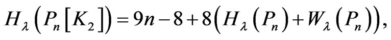
and

Remark 2.8. In Theorem 2.6, if , then we obtain
 , which gives first derivatives formula Theorem 5 in [22] at
 .
.
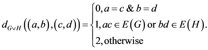
Now we prove the theorem that characterizes the generalized degree distance of the disjunction of two graphs.
Theorem 2.9. Let  and
and  be two graphs. Then

Proof. According to definition of , we have the following relations:


and
So we have:

This completes the proof. □
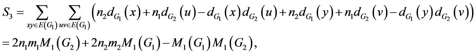
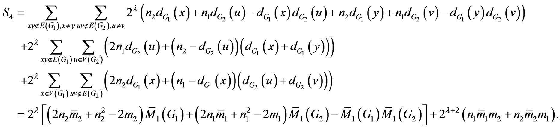
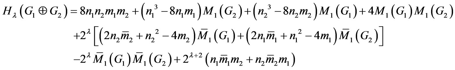
Now we prove the theorem that characterizes the generalized degree distance of the symmetric difference of two graphs.
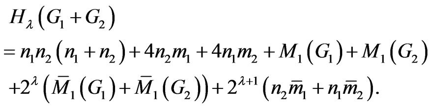
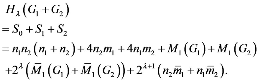
Theorem 2.10. Let G1 and G2 be two graphs. Then
Proof. We consider four sums  as follows:

similarly to 

and

By the definition of , we have:

So the proof is now completed. □
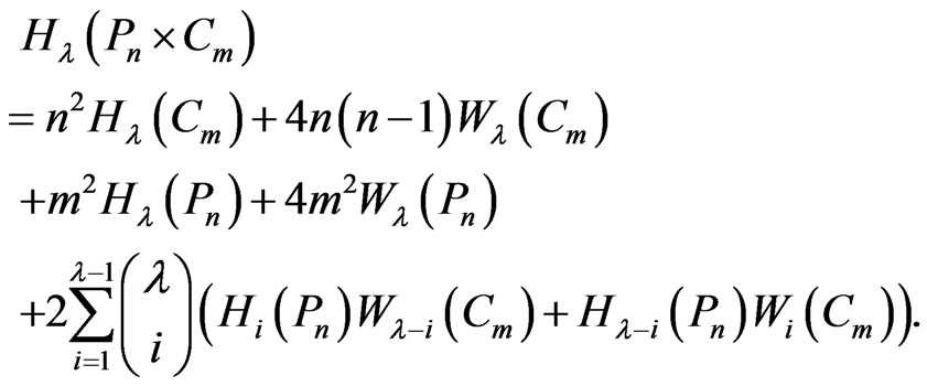
In the next theorem we find the generalized degree distance of the Cartesian product of two graphs.
Theorem 2.11. Let  and
and  be two graphs. Then

Proof. Suppose  and
and  are two set of vertices of
  and
and , respectively. Then by Lemma 2.1 and definition of
 , we have:

So the proof is now completed. □
As an application of the above theorem, we list explicit formulae for the generalized degree distance of  and
and . These graphs are known as the rectangular grid, the
  nanotube, and the
  nanotorus, respectively.
Lemma 2.12. Define . By [1,23], we have:

Corollary 2.13. By Theorem 2.9 and Lemma 2.12 we have:

and
Remark 2.14. In the above theorem, if , then we obtain
 , which gives first derivatives formula Theorem 1 in [22] at
 .
.
Now we obtain the relation between the generalized degree distance polynomial and Wiener-type invariant polynomial and the relation between the modified generalized degree distance polynomial and Wiener-type invariant polynomial for graphs.
Theorem 2.15. If  is a graph with
  vertices and
  edges, then
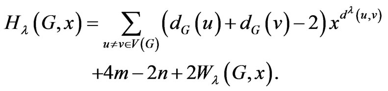
Proof. By definition, we have

This completes the proof. □
Theorem 2.16. If  is a graph with
  vertices and
  edges, then

Proof. By definition, we have

This completes the proof. □
NOTES