Existence and Uniqueness of Positive (Almost) Periodic Solutions for a Neutral Multi-Species Logarithmic Population Model with Multiple Delays and Impulses ()
1. Introduction
Recently, there are more works on the periodic solution of neutral type Logistic models or Lotka-Volterra models (see [2-7] for details). Only a little scholars considered the neutral Logarithmic model (see [1,8-10]). In [8], Li had studied the following single species neutral Logarithmic model:
 (1.1)
(1.1)
He had established a set of easily applicable criteria for the existence of positive periodic solution of system (1.1) by applying the continuation theorem of the coincidence degree theory which proposed in [11] by Mawhin. In [9], Lu and Ge employed an abstract continuous theorem of k-set contractive operator to investigate the following equation:
 (1.2)
(1.2)
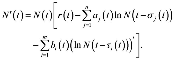
They established some criteria to guarantee the existence of positive periodic solutions of system (1.2). In [10], Chen studied the following neutral multi-species Logarithmic population model:
 (1.3)
(1.3)
By using the method of fixed point theory and constructing a suitable Lyapunov functional, a set of easily applicable criteria are established for the existence, uniqueness and global attractivity of positive periodic solution (positive almost periodic solution) for system (1.3).
In [1], Wang et al. had investigated the existence, uniqueness of the positive periodic solution of the following neutral multi-species Logarithmic population model:
 (1.4)
(1.4)
By using an abstract continuous theorem of k-set contractive operator, the criteria is established for the existence, global attractivity of positive periodic solutions for model (1.4).
On the other hand, there are some other perturbations in the real world such as fires and floods that are not suitable to be considered continually. These perturbations bring sudden changes to the system. Systems with such sudden perturbations involving impulsive differential equations have attracted the interest of many researchers in the past twenty years [12-20], since they provide a natural description of several real processes subject to certain perturbations whose duration is negligible in comparison with the duration of the process. Such processes are often investigated in various fields of science and technology such as physics, population dynamics, ecology, biological systems, optimal control, etc. For details, see [21,22]. Recently, the corresponding theory for impulsive functional differential equations has been studied by many authors [23-25]. However there are few published papers discussing the impulsive neutral multispecies Logarithmic population model. Our method is different from that in [1,9].
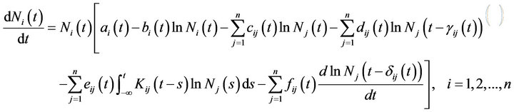
In this paper, we investigate the existence, uniqueness of the positive periodic solution of the following neutral multi-species Logarithmic population system with multiple delays and impulses
 (1.5)
(1.5)
where 


 are all continuous functions with
 ,
,  ,
, . And
. And ,
,  ,
, . We consider (1.5) together with the initial conditions
 (1.6)
(1.6)
For the ecological justification of (1.5) and the similar types refer to [1,8-10].
Throughout this paper, we make the following notations:
Let  be a constant and
 with the norm defined by
 ;
;
 with the norm defined by
 .
.
Then  are Banach spaces.
For the sake of generality and convenience, we always make the following fundamental assumptions:
(H1) ,
,  ,
,  ,
,  ,
,  , are all positive periodic continuous functions with period
 , and
, and  are positive continuously differentiable
  -periodic functions. Furthermore,
  ,
,  are positive
  - periodic continuous functions such that
 ,
,  , and
, and  exists;
(H2)  are fixed impulsive points with
 ;
;
(H3)  is a real sequence such that
 ,
,  is an
is an  -periodic function;
(H4) ,
,  ,
,  ,
,  ,
,  , are all almost periodic continuous functions with period
  on R, and
  are positive continuously differentiable almost periodic functions such that

where

(H5) ,
,  are positive continuously differentiable almost periodic functions such that
 ,
,  , and
, and  exists,
  are fixed impulsive points with
 ;
;
(H6)  is a real sequence such that
 ,
,  is an almost periodic continuous function.
The outline of the paper is as follows. In the following section, some definitions and some useful lemmas are listed. In the third section, we first introduce a transformation, where some adjustable real parameters  0 are introduced. After that, by using contraction mapping principle, we derive some sufficient conditions which ensure the existence and uniqueness of positive periodic solution (positive almost periodic solution) of system (1.5) and (1.6). In the fourth section, we derive a set of easily verifiable criteria for the global attractivity of the positive periodic solution (almost periodic solution) of (1.5) and (1.6) by constructing a suitable Lyapunov functional. Finally, we give an example to show our results. Here, We must point out, the idea of introducing parameters is stimulated by the recent works of [1,26, 27]. However, to the best of the authors knowledge, this is the first time such a technique is applied to the impulsive neutral delays ecosystem.
2. Preliminaries
In order to obtain the existence and uniqueness of a periodic solution for system (1.1) and (1.2), we first give some definitions and lemmas:
Definition 2.1 ([21]) A function  is said to be a positive solution of (1.5) and (1.6), if the following conditions are satisfied:
1)  is absolutely continuous on each
2) for each 
 and
and  exist and
3)  satisfies the first equation of (1.1) and (1.2) for almost everywhere (for short a.e.) in
  and satisfies
 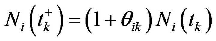 for
for ,
,  .
.
Definition 2.2 Let  be a strictly positive periodic solution (almost periodic solution) of (1.5) and (1.6). We say
  is globally attractive if any other solution
  of (1.5) and (1.6) has the property:

We can easily get the following Lemma 2.1.
Lemma 2.1 The region
 is the positive invariable region of the system (1.5).
Proof. In view of biological population,we obtain  By the system (1.5), we have

and


Then the solution of (1.5) is positive.
Under the above hypotheses (H1)-(H3), I consider the neutral non-impulsive system
 (2.1)
(2.1)
with initial conditions:
 (2.2)
(2.2)
where
 (2.3)
(2.3)
By a solution  of (2.1) and (2.2), it means an absolutely continuous function
 ,
,  , defined on
  that satisfies (2.1) a.e., for t ≥ 0, and
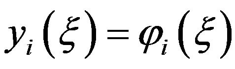 ,
,  on
on .
.
The following lemmas will be used in the proofs of our results, The proof of the first lemma is similar to that of Theorem 1 in [20].
Lemma 2.2 Suppose that (H1)-(H3) hold. Then 1) if  is a solution of (2.1) and (2.2) on
 , then

is a solution of (1.5) and (1.6) on .
.
2) if  is a solution of (1.5) and (1.6) on
 , then

is a solution of (2.1) and (2.2) on .
.
Proof. Its proof is similar to that of Theorem 1 in [20], here we omit it.
Lemma 2.3 ([28]) Suppose  and
and ,
, . Then the function
  has a unique inverse
  satisfying
  with
with 

Proof. Its proof is similar to that of Lemma 2.4 in [29], here we omit it.
Lemma 2.4 (Barbalat’s Lemma [30]) Let  be a nonnegative function defined on
  such that
  is integrable and uniformly continuous on
 , then
 .
.
Lemma 2.5 Assume that ,
,  are all continuously differentiable
  -periodic functions,
  ,
,  are both nonnegative continuous
  -periodic functions such that
 , then
where 
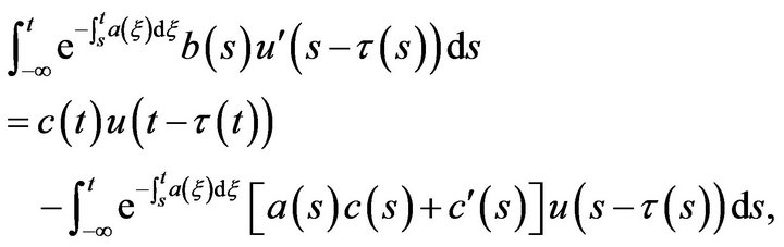
Proof. As
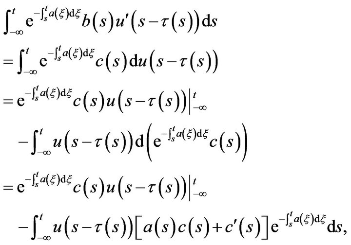 (2.4)
(2.4)
Denote , then from
 ,
,
 it follows m < 1. Also, when t ≥ s without loss of generality, we may assume
  , thus

Therefore

and so, from (2.9) it follows:

The proof is complete. 
Lemma 2.6 Assume that  are all continuously differentiable almost periodic functions,
  are both nonnegative continuous almost periodic functions such that
 ,
,  is positive number, then

where 
Proof. Similar to the proof of Lemma 2.5, we omit it here.
3. Main Theorem
Here, we take the transformation , then (2.1) can be rewritten in the following form
 (3.1)
(3.1)
Obviously, the existence, uniqueness and global attractivity of positive periodic solution (almost periodic solution) of system (1.5) is equivalent to the existence, uniqueness and global attractivity of periodic solution (almost periodic solution) of system (3.1).
For , let us consider the equation
 (3.2)
(3.2)
Since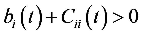 ,
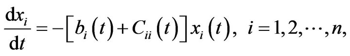
,  , it follows that the linear system of system (3.2)
 (3.3)
(3.3)
admits exponential dichotomies on R, and so, system (3.3) has a unique continuous periodic solution , which can be expressed as
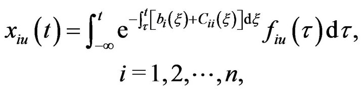 (3.4)
(3.4)
where
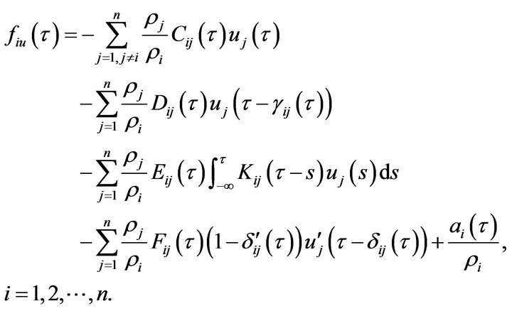 (3.5)
(3.5)
Now, by using Lemma 2.5,  can also be expressed as
 (3.6)
(3.6)
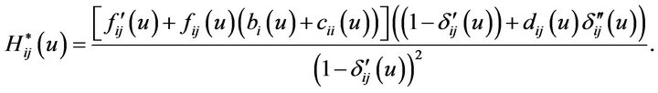
where
 (3.7)
(3.7)
Our main result on the global existence of a positive periodic solution of (1.5) and (1.6) is stated as follows.
Theorem 3.1 In addition to (H1)-(H3), assume further that there exist positive constants , such that
(H7) 
Then (1.5) has a unique positive  -periodic solution with strictly positive components, say
 where
where

and

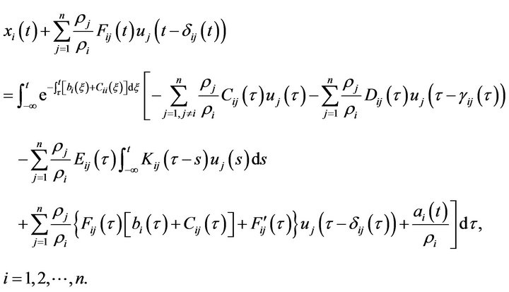
Proof. For , from (3.6), we know that
 (3.8)
(3.8)
where  are defined by (3.7), is a continuous
  - periodic function, and so
 . Now define the mapping
  as follows:
 (3.9)
(3.9)
Following we will prove the mapping  is a contraction mapping. In fact, for any
 and
and
 from (3.8), (3.9) and the conditions of Theorem 3.1 it follows:
 (3.10)
where

That is
 (3.11)
This shows that  is a contraction mapping. Hence, there exists a unique fixed point
  such that
 , that is
 (3.12)
Following, we prove  is the periodic solution of system (3.1). Noticing that (3.12) is equivalent to
 (3.13)
From the right-hand sides of (3.13), we know that

is differentiable. And so, from (3.13) it follows that

here using the equality (3.13) again. That is
 (3.14)
This shows that  is continuously differentiable
  -periodic function and satisfies Equation (3.1). Therefore,
  is the unique continuously differentiable
  -periodic solution of system (3.1), and so,

is the unique positive  -periodic solution of system (2.1), from Lemma 2.2,

is the unique positive  -periodic solution of system (1.5). The proof is complete.
As a direct corollary of Theorem 3.1, one has Corollary 3.1 In addition to (H1)-(H3), assume further that there exist positive constants , such that

Then (1.5) has a unique positive  -periodic solution with strictly positive components.
Our next theorem concerned with the existence of unique positive almost periodic solution of systems (1.5) and (1.6).
Let  be any continuously differentiable almost periodic function, and consider equation,
 (3.15)
Since , it follows that the linear system of system (3.15)
 (3.16)
admits exponential dichotomies on R, and so, system (3.16) has a unique continuous almost periodic solution , which can be expressed as
 (3.17)
where
 (3.18)
Now, by using Lemma 2.5,  can also be expressed as
 (3.19)
where
 (3.20)
Then, we have Theorem 3.2 In addition to (H4)-(H6), assume further that there exist positive constants , such that
(H8) 
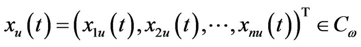
Then (1.5) has a unique positive almost periodic solution with strictly positive components, say
 where
where

and

Proof. Set

with the norm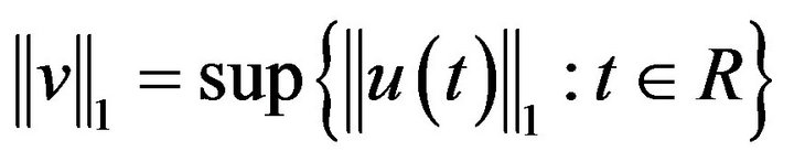 , obviously, C is a Banach space. For any continuously almost periodic function
  we know that
  defined by (3.19) is also a continuously almost periodic function. Now define the mapping
  as follows:
 (3.21)
Then similarly to the prove of Theorem 3.1, we could prove that under the assumptions of Theorem 3.2, the mapping  is a contract mapping, and so system (3.19) has a unique fixed point
 . and so,

is the unique positive almost periodic solution of system (2.1), from Lemma 2.2,

is the unique positive almost periodic solution of system (1.5). The proof is complete. 
As a direct corollary of Theorem 3.2, one has Corollary 3.2 In addition to (H4)-(H6), assume further that there exist positive constants , such that

Then (1.5) has a unique positive almost periodic solution with strictly positive components.
Consider the following equation:
 (3.22)
which is a special case of system (1.5) and (1.6) without impulse. Similarly, we can get the following results.
Theorem 3.3 In addition to (H1), assume further that there exist positive constants , such that
(H9) 
Then (1.5) has a unique positive  -periodic solution with strictly positive components, say
 .
.
where

and

Proof. Similar to the proof of Theorem 3.1, we omit it here.
As a direct corollary of Theorem 3.3, one has Corollary 3.3 In addition to (H1), assume further that there exist positive constants , such that

Then (1.5) has a unique positive  -periodic solution with strictly positive components.
Theorem 3.4 In addition to (H4), assume further that there exist positive constants , such that
(H10) 
Then (1.5) has a unique positive almost periodic solution with strictly positive components, say
 .
.
where

and

As a direct corollary of Theorem 3.4, one has Corollary 3.4 In addition to (H4), assume further that there exist positive constants , such that

Then (1.5) has a unique positive almost periodic solution with strictly positive components.
4. Global Asymptotic Stability
In this section, we devote ourselves to the study of the global attractivity of periodic solutions (almost periodic solutions) of system (1.5), (1.6) and (3.22) (which is a special case of system (1.5) and (1.6) without impulse). Now, we state our main results of this section as follows:
Theorem 4.1. Assume that the conditions in Theorem 3.1 hold. Suppose further the following conditions hold:
(H11) There is a positive constant M such that

(H12) 
Then system (1.5) and (1.6) has a unique periodic solution which is globally attractive.
Proof. Let  be the unique positive periodic solution of system (1.5) and (1.6)whose existence and uniqueness are guarantee by Theorem 2.1, and
  be any other solution of system (1.5) and (1.6). Let

then, similar to Equation (3.1), we have
 (4.1)
(4.1)
and,
 (4.2)
(4.2)
Then, from (4.1) and (4.2), we have
 (4.3)
(4.3)
Let , then
 (4.4)
(4.4)
Multiply both sides of (4.4) with  and then integrate from 0 to
  to obtain
 (4.5)
(4.5)
then
 (4.6)
(4.6)
thus
 (4.7)
(4.7)
Let , by Lemma 2.3, we obtain
 (4.8)
(4.8)
where

Thus,
 (4.9)
(4.9)
then
 (4.10)
That is
 (4.11)
From (H3), we have
 (4.12)
From (H4), we have
 (4.13)
thus,  that is the positive
  -periodic solution of (3.1) is globally attractive,

by Definition 2.2, the positive  -periodic solution of (1.5) is globally attractive. The proof is completed.
Theorem 4.2. Assume that the conditions in Theorem 3.2 hold. Suppose further the following conditions hold:
(H13) There is a positive constant m such that

(H14) 
Then system (1.5) and (1.6) has a unique almost periodic solution which is globally attractive.
Proof. Similar to the proof of Theorem 4.1, we omit it here.
Theorem 4.3. Assume that the conditions in Theorem 3.3 (or Theorem 3.4) hold. Suppose further the following conditions hold:
(H15) There is a positive constant  such that

(H16) 
Then system (3.22) has a unique periodic solution (almost periodic solution) which is globally attractive, where
Proof. Similar to the proof of Theorem 4.1, we omit it here.
5. An Example
Now, we give an example to demonstrate our result. Let us consider the following equation:
 (5.1)
(5.1)
Compare with (3.22), we get ,
, 

 ,
, 


So, 


 and
and
 (5.2)
(5.2)
According to Corollary 3.3, we see that system (5.1) has at least one positive  -periodic solution.
6. Acknowledgements
This work was supported by the construct program of the key discipline in Hunan province.
NOTES
#Corresponding author.