1. Introduction
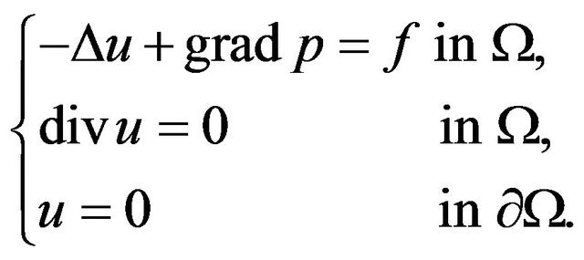
Concerned with the perturbed Navier-Stokes equations:
 (1.1)
(1.1)
where  is a smooth bounded domain with boundary
 , and p, u is the velocity vector,
  is the pressure at x at time t, and
  is the kinematic viscosity, and f represents volume forces that are applied to the fluid, and
 , where
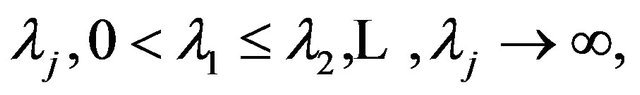
  is the first eigenvalue of A (see Remark 4). The Equation (1.1) is Navier-Stokes equations, as
 , which show the existence of absorbing sets and the existence of a maximal attractor, the universal attractor, attractor in unbounded domain (see [1-5]). ACTA Mathematical Application Sinica. In [6], where they some interesting results, as
 . In [7,8] Babin, Vishik and Abergel consider maximal attractors of semigroups corresponding to evolution differential equations, existence and finite dimensionality of global attractor for evolution equations on unbounded domains. In [9,10] A. Pazy consider Semigroups of linear operator and application to partial differential equation.
We need the following preliminaries:
Equations (1.1) are supplemented with a boundary condition. Two cases will be considered: The nonslip boundary condition. The boundary  is solid and at rest; thus
 (1.2)
(1.2)
The space-periodic case. Here  and
and
 (1.3)
(1.3)
Remark 1. If  is solid but not rest, then the nonslip boundary condition is
  on
on  where
where  is the give velocity of
 .
.
Remark 2. That is u and p take the same values at corresponding points of .
.
Furthermore, we assume in this case that the average flow vanishes
 (1.4)
(1.4)
When an initial-value problem is considered we supplement these equations with
 (1.5)
(1.5)
For the mathematical setting of this problem we consider a Hilbert space H (see [8]) which is a close subspace of  (
( here).
In the nonslip case,
 (1.6)
(1.6)
and in the periodic case
 (1.7)
(1.7)
We refer the reader to R. Temam [2] for more details on these spaces and, in particular, a trace theorem showing that the trace of  on
on  exists and belong to
  when
when  and
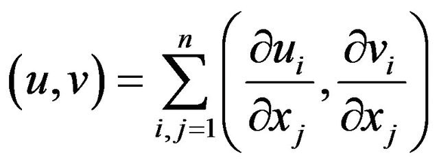
and . The space H is endowed with the scalar product and the norm of
  denoted by
  and
and .
.
Remark 3.  and
and  are the faces
  and
and
 of
of . The condition
  expresses the periodicity of
 ;
;  is the space of
  satisfying (1.4).
Another useful space is  a closed subspace of
 (1.8)
(1.8)
in the nonslip case and , in the space-periodic case,
 (1.9)
(1.9)
where  is define in [1]. In both case, v is endowed with the scalar product
and the norm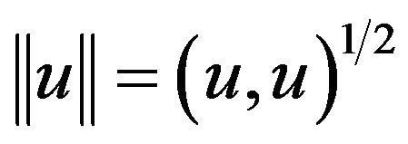 .
.
We denoted by A the linear unbounded operator in H which is associated with V, H and the scalar product ,
, . The domain of A in H is denoted by
 ; A is self-adjoint positive operator in H. Also A is an isomorphism from
  onto H. The space
  can be fully characterized by using the regularity theory of linear elliptic systems (see [1,3]).
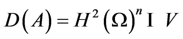
and  in the nonslip and periodic cases; furthermore,
  is on
is on  a norm equivalent to that induced by
  Let
Let  be the dual of V; then H can be identified to a subspace of
  and we have
 (1.10)
where the inclusions are continuous and each space is dense in the following one.
Remark 4. In the space-periodic case we have 
 ,
,  , while in the nonslip case we have
 ,
,  , where P is the orthogonal projector in
  on the space H. We can also say that
  is equivalent to saying that there exists
  such that
The operator  is continuous from H into
  and since the embedding of
  in
in  is compact, the embedding of V in H is compact. Thus
  is a self-adjoint continuous compact operator in H, and by the classical spectral theorems there exists a sequence
and a family of elements  of
of  which is orthonormal in H, and such that
 (1.11)
We need the following main Result:
Lemma 1.1. (see [4]) (Uniform Gronwall Lemma) Let  be three positive locally integrable function on
  such that
  is locally integrable on
 , and satisfy
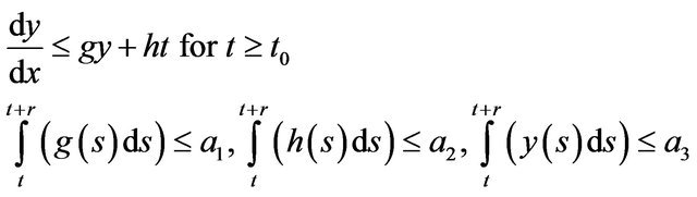
for  where
where 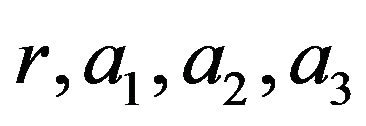 are positive constant. Then
 .
.
The evolution of the dynamical system is described by a family of operators , that map H into itself and enjoy the usual semigroup properties (see [8]):
 (1.12)
 (1.13)
The operator  are uniformly compact for t large. By this we mean that for every bounded set X there exists
  which may depend on X such that
 (1.14)
for every bounded set ,
,
 (1.15)
Of course, if H is Banach space, any family of operators satisfying (1.14) also satisfies (1.15) with .
.
Theorem 1.2. (see [4]) We assume that H is a metric space and that the operators  are given and satisfy (1.12), (1.13) and either (1.14) or (1.15). We also assume that there exists an open set
  and abounded set X of
  such that X is absorbing in
 . Then w-limt set of
 , is a compact attractor which attracts the bounded set of
 . It is the maximal bounded attractor in
  (for the inclusion relation). Furthermore, if H is a Banach space, if U is convex2, and the mapping
  is continuous from
 , for every
  in H; then
  is connected too.
The rest of this paper is organized such that Section 2 contains a sketch of existence and uniqueness of solution of the equations; in Section 3 we show the existence of absorbing set and the existence of a maximal attractor; in Section 4 contain the proof of existence and uniqueness of solution of the equations, in Section 5 discussed the perturbation coefficients .
.
2. Existence and Uniqueness of Solution of the Equations
The weak from of the Navier-Stokes equations due to J. Leray [1-3] involves only u, as . It is obtained by multiply (1.1) by a test function v in V and integrating over
 . Using the Green formula (1.1) and the boundary condition, we find that the term involving p disappears and there remains
 (2.1)
(2.1)
where
 (2.2)
(2.2)
whenever the integrals make sense. Actually, the from b is trilinear continuous on  and in particular on V. We have the following inequalities giving various continuity properties of b:
 (2.3)
(2.3)
where  is an appropriate constant
 .
.
An alternative from of (2.1) can be given using the operator  and the bilinear operator
  from
from  into
into  defined by
 (2.4)
(2.4)
we also set

and we easily see that (2.1) is equivalent to the equation
 (2.5)
(2.5)
while (1.5) can be rewritten
 (2.6)
(2.6)
We assume that f is in dependent of  so that the dynamical system associated with (2.5) is autonomous
 (2.7)
(2.7)
Existence and uniqueness results for (2.5) (2.6) are well know as  (see [2,3]). The following theorem collects several classical results.
Theorem 1.3. Under the above assumption, for  and
and  given in
  t here exists a unique solution
  of (2.4) (2.5) satisfying
 ; Furthermore,
  is analytic in
  with values in
  for
for , and the mapping
  is continuous from
  into
into ; Finally, if
 , then
 . Some indications for the proof of Theorem 1.3 will be given in Section 4. This theorem allows us to define the operators
These operator enjoy the semigroup properties (1.12) and the are continuous from H into itself and even from H into .
.
3. Absorbing Sets and Attractor
The part proof about global attractor is similar to the Temam’s book, but the exists of perturbation term is different from the Temam’s book, so we reprove it for integrality.
Theorem 1.4. The dynamical system associated with the tow-dimensional modified Navier-Stokes equations, supplemented by boundary (1.2) or (1.3), (1.4) possesses an attractor  that is compact, connected,and maximal in H.
  attracts the bounded sets of H and
  is also maximal among the functional invariant set bounded in H.
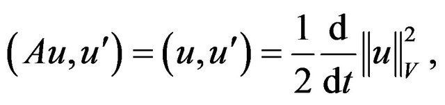
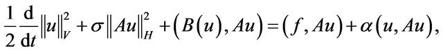
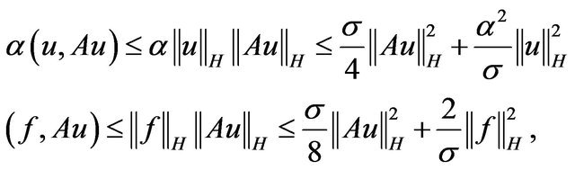
Proof. We first prove the existence of an absorbing set in H. A first energy-type equality is obtained by taking the scalar product of (2.5) with . Hence
 (3.1)
(3.1)
We see that  and there remains
 (3.2)
(3.2)
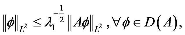
We know that  where
where  is the first eigenvalue of
 . Hence, we can majorize the right-hand side of (3.1) by

the estimates 
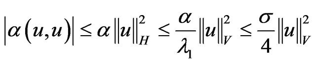
Hence we obtain
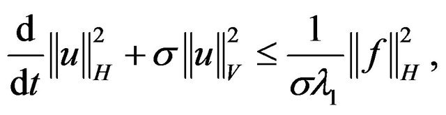 (3.3)
(3.3)
 (3.4)
(3.4)
Using the classical Gronwall Lemma, we obtain
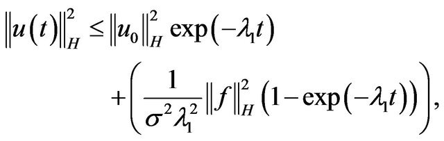 (3.5)
(3.5)
Thus
 (3.6)
(3.6)
We infer (3.5) that the ball  of
of  with
with  are positively invariants for the semigroup
 , and these balls are absorbing for any
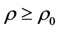 . We choose
  and included a ball
  of
of , It is easy to deduce from (3.5) that
  for
for , where
 (3.7)
(3.7)
We the infer from (3.3), after integration in t, that
 (3.8)
(3.8)
With the use of (3.6) we conclude that
 (3.9)
(3.9)
and if  and
and , then
 (3.10)
1) Absorbing set in V An continue and show the existence of an absorbing set in V. For that purpose we obtain another energy-type equation by taking the scalar product of (2.5) with . Since
we find
we writer
and using the second inequality (2.3)
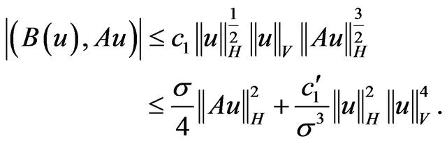
Hence
 (3.12)
and since
 (3.13)
We also have
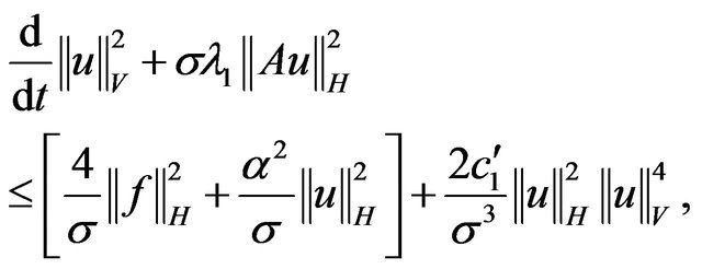 (3.14)
We a priori estimate of  follows easily from (3.14) by the classical Gronwall lemma, using the previous estimates on u. We are more interested in an estimate valid for large t. Assuming that
  belong to a bounded set X of H and that
  as in (3.7), we apply the uniform Gronwall lemma to (3.14) with
  replaced by
Thanks to (2.14), (2.18) we estimate the quantities  in Lemma 1.1 by
 (3.15)
and we obtain
 (3.16)
 as in (3.7). Let us fix
  and denote by
  the right-hand side of (2.24). We the conclude that the ball
  of V, denoted by X1, is an absorbing set in V for the semigroup
 . Furthermore, if X is any bounded set of H, then
  for
for . This shows the existence of an absorbing set in V, namely X, and also that the operators
  are uniformly compact, i.e., Theorem 1.1 is satisfied.
2) Maximal attractor All the assumption of Theorem 1.1 are satisfied and we deduce from this theorem the existence of a maximal attractor for modified Navier-Stokes equations. 
4. Proof of Theorem 1.3
The existence of a solution of (2.4) (2.5) that belong to , is first obtain by the Faedo-Gakerkin (see [3]) method. We implement this approximation procedure with the function
  representing the eigenvalues of A (see Remark 4). For each m we look for an approximate solution
  of the form
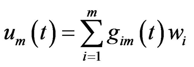
satisfying
 (4.1)
(4.1)
 (4.2)
(4.2)
where  is projector in H (or V) on the space spanned by
 . Since A and
  commute, the relation (3.1) is also equivalent to
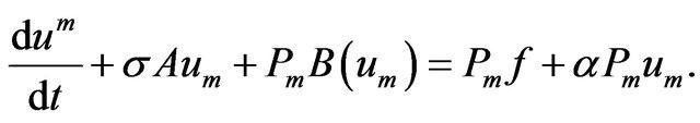 (4.3)
(4.3)
We prove  on
on  is Lip continuous,

hence
there is m, M such that . When
  is established, and when
  is established, then
On both sides in the integral , then
we writer

Hence  on
on  is Lip continuous. The existence and uniqueness of
  on some interval
  is elementary and then
 , because of the a priori estimates that we obtain for
 . An energy equality is obtained by multiplying (4.1) by
  and summing these relations for
 . We obtain (3.2) exactly with u replaced by
  and we deduce from this relation that
 (4.4)
(4.4)
Due to (3.1) and the last inequality (2.3)
 (4.5)
(4.5)
Therefor  and
and  remain bounded in
  and by (4.3)
 (4.6)
(4.6)
By weak compactness it follows from (4.3) that there exists , and a subsequence still denoted m, such that
 (4.7)
(4.7)
Due to (4.6) and a classical compactness theorem (see [2]), we also have
 (4.8)
(4.8)
This is sufficient to pass to the limit in (4.1)-(4.3) and we find (2.4), (2.5) at the limit. For (2.5) we simply observe that (4.7) implies that  weakly in
  or even in
 .
.
By (2.4),  belong to
  and, u is in
 . The uniqueness and continuous dependent of
  on
on  (in
(in ) follow by standard using [2].
The fact that , is proved by deriving further a priori estimates on
 . They are obtained by multiplying (4.1) by
  and summing these relations for
 . Using (1.11) we find a relation that is exactly (3.11) with
  replaced by
 . we deduce form this relation that
 (4.9)
(4.9)
At the limit we then find that u is in . The fact that u in
  then follows from an appropriate application of Lemma 3.2 [2].
Finally, the fact that u is analytic in t with values in  results from totally different methods, for which the reader is referred to C. Foias and R. Temam [1] or R. Temam [3]. However, this property was given for the sake of completness and is never used here in an essential manner.
5. The Limit-Behavior of Navier-Stokes Equation with Nonlinear Perturbation
We consider the limit-behavior of Navier-Stokes equation with nonlinear perturbation on the two dimensional space. we use the space which is given (1.6), (1.8). The main advantage we see is that applying the Gronwall lemma to the solution of problem (1.1) approaches a solution of Navier-Stokes equation on  and
and , as
, as .
.
Theorem 1.6. Under assumption (1.6), then the solution of  of (1.1) is approximate solution of Navier-Stokes equations and this solution is stable, as
 .
.
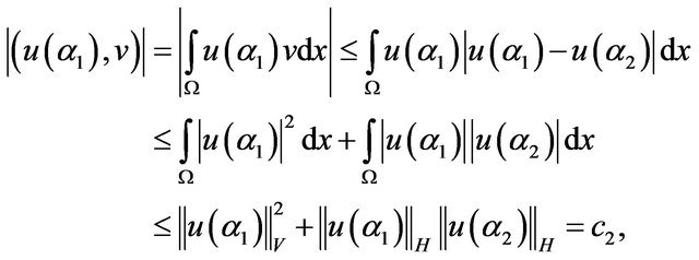
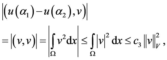
Proof. Let  is a solution of (1.1), as
 :
:
 (5.1)
(5.1)
Let  is a solution of (1.1), as
 :
:
 (5.2)
(5.2)
Utilizing (5.1)-(5.2) and let  Hence
Hence
 (5.3)
(5.3)
It is obtained by multiply (5.4) by a function  in
in  and integrating over
 .
.
 (5.4)
(5.4)
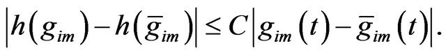
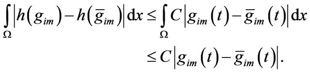
Using the second inequality (2.3) and  is trilinear continuous:
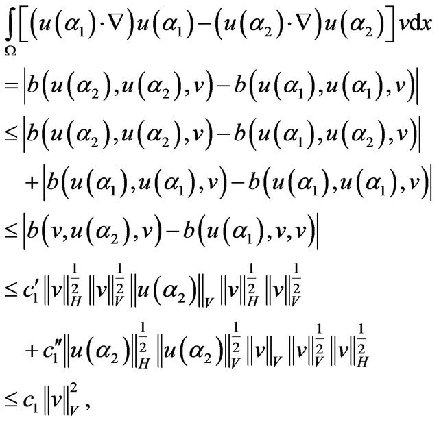
and
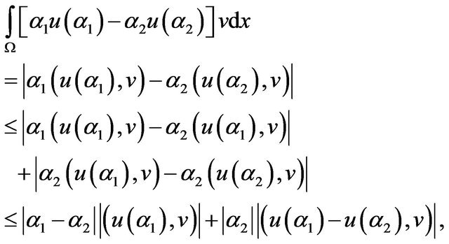
utilizing inequality (**), (3.6), (3.46) we estimate 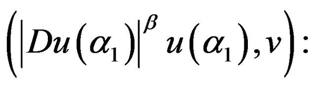
we write
hence
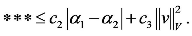
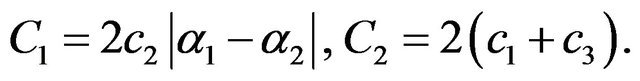
where  is an appropriate constant. Hence
 (5.5)
(5.5)
i.e.
 (5.6)
(5.6)
Using the classical Gronwall Lemma, we obtain
 (5.7)
(5.7)
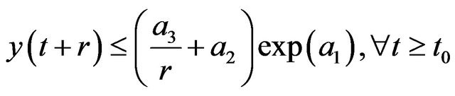
where
Notice that  Thanks to
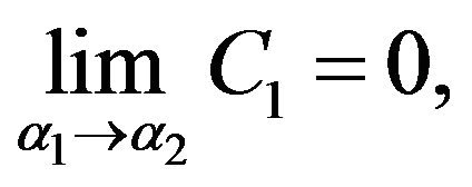
hence

Hence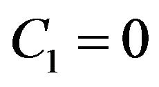 ,
,  as
as , according to stable condition, thus this solution is stable.
NOTES
#Corresponding author.