Derivation the Schemes of Lateral and Vertical Dispersion Parameters: Application in Gaussian Plume Model ()
1. Introduction
The study and employment of operational short-range atmospheric dispersion models for environmental impact assessment have demonstrated to be of large use in the evaluation of ecosystems perturbation in many distinct scales [3].
In operational applications, the classical Gaussian diffusion models are largely employed in assessing the impacts of existing and proposed sources of air contaminants on local and urban air quality [4]. Simplicity, associated with the Gaussian analytical model, makes this approach particularly suitable for regulatory usage in mathematical modeling of the air pollution, such models are quite useful in short forecasting. The lateral and vertical dispersion parameters, respectively σy and σz represent the key turbulent parameterization in this approach. They contain the physical ingredients that describe the dispersion process and, consequently, express the spatial extent of the contaminant plume under the effect of the turbulent motion in the planetary boundary layer (PBL) [5].
In this work, we estimated the schemes of dispersion parameters in the lateral direction (σy) and the vertical direction (σz) in unstable stability by using wind speed in power law and comparing between our work and da (algebraic and integral formulations) with observed ta of sulfur hexafluoride (SF6) are taken from Copenhagen in Denmark.
2. Model Formulation
The concentration associated from point source of strength Q, is expressed as [6]:
 (1)
(1)
C is the average concentration of diffusing point (x, y, z) (kg/m3).
U is mean wind velocity along the x-axis (m/s).
x is along-winds coordinate measured in wind direction from the source (m).
y is cross-wind coordinate direction (m).
z is vertical coordinate measured from the ground (m).
σy is the plume dispersion parameter in the lateral directions.
Where the value of the parameter, s, depends on the stability (s = 0.75 and A = 1.42) in unstable case [7].
The mean plume height,  , is defined by
 (2)
(2)
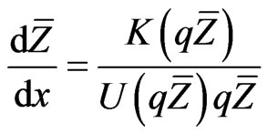
And the mean plume velocity,  , is defined by
 (3)
(3)
We assume that the mean wind speed, U(z), can be described by a power law so that:
 (4)
(4)
Ur is a reference velocity at height Zr, the value of the power, p, lies between 0.15 and 0.20 in unstable case [8].
Let, B, be a non-zero constant, then taking:
 (5)
(5)
Substitution from equations (1) and (5) in equation (2) one gets:
 (6)
(6)
where Г (p) is the gamma function.
Substituting from Equations (4), (1) and (5) in Equation (3), we obtain the mean plume velocity:
 (7)
(7)
The mean plume height,  , can be calculated according to [9]:
 (8)
(8)
and
 (9)
(9)
where K(z) is the eddy diffusivity parameterization that is led to the K-theory assumption.
According to [10], the form of K(z) in an unstable case is:
 (10)
(10)
where k is the Von Karman constant which is set to 0.4, w* is the convection scaling parameter and h is the effective height of release above the ground estimated from [11]:

where hs is physical stack height (115m).

where, W, is the exit velocity (4 m/s), D is the internal stack diameter (1 m) and
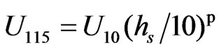
U10 is the wind speed at 10 m height.
Substituting from equations (4), (10) in Equation (8) and integrating equation (8), we obtain the mean plume height :
:
 (11)
(11)
Substituting from Equation (11), in Equation (7), we obtain the mean plume velocity :
:
 (12)
(12)
We estimate the horizontal spread σy using Eckman’s (1994) hypothesis that [12]:
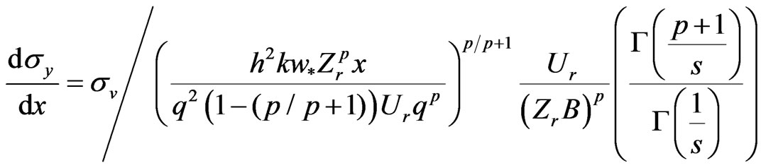 (13)
(13)
where

where σv is the standard deviation of the wind speed in the lateral direction.
By Integrating the equation (13) with respect to x, we obtain the plume dispersion parameter in the lateral direction (σy) as follows:

Also estimating the vertical spread σz using hypothesis by [12]:
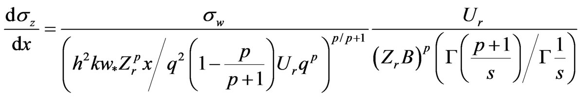 (15)
(15)
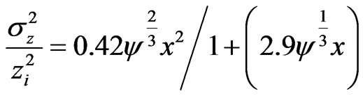
where σw is the standard deviation of the wind speed in the vertical direction. Integrating Equation (15) with respect to x, we obtain the plume dispersion parameter in the vertical direction (σz) as follows:
 (16)
(16)
Then Gaussian expressions for the ground crosswind integrated concentration and the normalized ground level concentration along the plume centerline respectively are given by [4] on the forms:
 (17)
(17)
 (18)
(18)
From the previous works, the plume dispersion parameters in the vertical and lateral directions (σz and σy) respectly are given by [1] in the form:
 (19)
(19)
and
 (20)
(20)
Also, the plume dispersion parameters in the vertical and lateral directions (σz and σy) respectively are given by [2] as follows:
 (21)
(21)
 (22)
(22)
3. Results and Discussion
The used data set was observed from the atmospheric diffusion experiments conducted at the northern part of Copenhagen, Denmark, under unstable conditions [13] and [14]. The tracer sulfur hexafluoride (SF6) was released from a tower at a height of 115 m without buoyancy. There are two Gaussian models. The First is measured at ground surface and the other at the plume centerline. In this work, there are three predicated normalized concentrations (our model and two previous models) as shown in Tables 1 and 2.
Figures 1 and 2 show that the observed and predicated scatter diagram of crosswind integrated concentrations of centerline and ground level respectively using Gaussian model with vertical and lateral dispersion parameters given by (Equations (14) and (16) our model) and (Equations (19) and (20), algebraic formulation), (Equations (21) and (22), integral formulation) respectively. From the two figures one finds that there are some predicated data which are agreement with observed data (one to one) and others lie inside the factor of two.
4. Statistical Method
Now, the statistical method is presented and comparison among analytical, statically and observed results will be offered [Hanna 1989, 15]. The following standard statistical performance measures that characterize the agreement between prediction (Cp = Cpred/Q) and observations (Co = Cobs/Q):
Normalized mean square error (NMSE): It is an esti-

Figure 1. Observed and predicated ground crosswind integrated centerline concentration, normalized with emission Cy(x, 0, 0)/Q: scatter diagram for the solution of Equation (18) using Equations (14), (16) and (19)-(22).

Figure 2. Observed and predicated ground crosswind integrated concentration, normalized with emission Cy(x, 0)/Q: scatter diagram for the solution of Equation (17) using Equations (16), (19) and (21).

Table 1. Observed and model ground-level centerline concentration. C(x, 0, 0)/Q at different distances, wind speed and effective height from the source.

Table 2. Observed and model ground-level concentration Cy(x, 0)/Q at different distances, wind speed and effective height from the source.
mator of the overall deviations between predicted and observed concentrations. Smaller values of NMSE indicate a better model performance. It is defined as:
 (23)
(23)
Fractional bias (FB): It provides information on the tendency of the model to overestimate or underestimate the observed concentrations. The values of FB lie between −2 and +2 and it has a value of zero for an ideal model. It is expressed as:
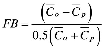 (24)
(24)
Correlation coefficient (R): It describes the degree of association between predicted and observed concentrations and is given by:
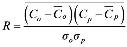 (25)
(25)
Fraction within a factor of two (FAC2) is defined as:


where σp and σo are the standard deviations of Cp and Co respectively. Here the over bars indicate the average over all measurements (Nm). A perfect model would have the following idealized performance: NMSE = FB = 0 and COR = FAC2 = 1.0 of the entire journals, and not as an independent document. Please do not revise any of the current designations.
From the statistical method of Table 3, we find that the predicted concentrations for all models lie inside factor of 2 with observed data. Regarding to NMSE, we find that two previous works are better than our model. Regarding to FB and correlation coefficient of all models are agreement with observed data.
Table 4 shows that the predicted concentrations for all models lay inside factor of 2 with observed data. Regarding to NMSE, all the predicted concentrations are better to the observed data. Regarding to FB and correlation coefficient of all methods are agreement with observed data.
5. Conclusions
New schemes of dispersion parameters in the lateral direction (σy) and the vertical direction (σz) are estimated in unstable stability by using power law wind speed and calculating Gaussian plume model at ground and at plume centerline.
One used observed data of the tracer sulfur hexafluo-

Table 3. Comparison between different models groundlevel centerline concentration cy(x, 0, 0)/Q and observed concentrations.

Table 4. Comparison between different models groundlevel centerline concentration Cy(x, 0)/Q and observed concentrations.
ride (SF6) which was released from a tower at a height of 115m without buoyancy at the northern part of Copenhagen, Denmark, under unstable conditions [13,14]. There are two Gaussian models; The First is measured at ground surface and the other at the plume centerline. In this work, there are three predicated normalized concentrations (our model and two previous models).
From the (figures 1 and 2), one finds that there are some predicated data which are agreement with observed data (one to one) and others lie inside the factor of two From the statistical method, we find that the predicted concentrations for all models lie inside factor of 2 with observed data. Regarding to NMSE, all the predicted concentrations are agreement with the observed data. Regarding to FB and correlation coefficient of all methods agree to observed data.
NOTES