Mathematical Model of Non-Coherent-DLL Discriminator Output and Multipath Envelope Error for BOC (α, β) Modulated Signals ()
1. Introduction
This template, MP propagation is widely recognized as the main error source in GNSS systems. In fact, the presence of MP signals provokes tracking error in the DLL which is a code discriminator that utilizes Earlyminus-late correlators [1], and thus it causes ranging errors in positioning the receiver. The MP tracking performances depend on various signal and receiver parameters [2,3] like signal type of modulation scheme such as BOC [3] and Multiplexed BOC (MBOC) [4,5] modulations for Galileo signals and modernized GPS signals [6] and Binary Phase Shift Keying (BPSK) for GPS signals [6], pre-correlation bandwidth and filter characteristics [7], type of Pseudo Random Noise (PRN) code, relative amplitude of MP signal, number of MP signals, MP delay, chip spacing between correlators in the DLL loop, type of discriminator used for tracking [8]. The influence of MP as an error source has resulted in the development of different MP mitigation techniques. These techniques are typically categorized in terms of antenna design [9,10], improved discriminator architecture, and post-processing of discernible objects [11-13]. In discriminator-architecture design, various techniques are proposed in the literature. Performances of the classical techniques are compared in [14] under the assumption that only single MP exists. In reference [15] the authors have proposed the “Virtual MP based Technique” for short delay MP mitigation. This technique is valid in some cases and it is limited in other cases [16]. In reference [17,18], an analysis and design of discriminator code tracking algorithms has been done to prove that the Narrow Correlator (NC) [19] is still the optimum choice among the considered algorithms. On the other hand, various approaches are also proposed to estimate the parameters of MP signals such as delays, amplitudes and phases. The estimated MP signals are then eliminated to track only the Line of Sight (LOS) signal [20-26]. All these techniques have proved to have the optimal performances in MP environments. However, all of them require a lot of hardware resources. In addition to the MP effect, another limitation exists in BOC and MBOC modulated signals due to the presence of side peaks in Correlation Function (CF) and thus the presence of several passages by zero in the DLL-DC which complicates the operation of the tracking process. For this reason various techniques are proposed for side peaks’ cancelation. The most basic of them are built on the basis of the CF of BOC and MBOC signals [27-30]. Other techniques, based on the modification of the locally generated codes, are proposed in [31-34]. The majority of these methods are based on computational geometry of CF and DC which require the knowledge of the mathematical models of CF and DCs [35]. Several models Have been proposed in scientific literature. Indeed, the CF of BOC (α, α), which is function of a specified width, has been proposed in reference [36]. In reference [37] authors have proposed another model characterizing the CF for case BOC (pα, α) (p integer). The general model BOC (α, β) have been proposed in reference [38]. In the same reference, the authors have proposed two other models which characterize respectively coherent DC and coherent MP tracking error. However, these models are valid only for some categories of BOC (α, β) modulated signals. In addition, the latter models contain some typing errors that have been corrected in [39].
In the coherent code tracking process the operation of estimating the delay of the received signal is function of the phase estimated by the Phase Locked Loop (PLL). Indeed, if the carrier phase of the received signal is estimated, the code delay search is called coherent signal tracking. In contrast, if the carrier phase is ignored, the search is called non-coherent signal tracking. This later process is used in the majority of the receiver’s architectures. Hence, this paper is devoted to the modeling of the non-coherent DLL-DC and MP tracking errors of BOC (α, β) codes. The paper is organized as follows:
We present firstly the coherent DLL-DC and we derive the proposed non-coherent one. Secondly, we derive the proposed non-coherent MP tracking error model. Finally we end up by a comparison of the proposed models and the numerical ones based on computer implementations.
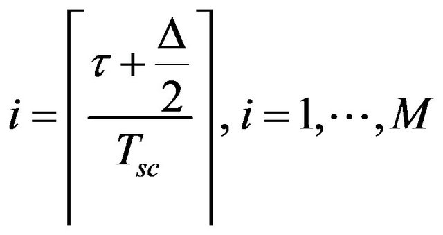
2. Coherent DLL-DC and the Proposed Non-Coherent
In the GNSS system the computation of the delay of the received signal is realized by the peak location of the CF, noted , between the received signal
  and the locally generated signal
 . This CF is given by the following equation:
 (1)
(1)
with:  is the time shift applied to the locally generated code.
BOC is a square waveform subcarrier modulation, where a signal  (the signal which is going to be modulated) is multiplied by a square waveform subcarrier of frequency
 . Formally, the BOC-modulated signal
  can be written as [3]:
 (2)
(2)
For GNSS signals, the notation BOC (α, β) is used, where α and β are two indices satisfying the relationships
 and
and 
where: fX is PRN code chipping rate.
BOC (α, α) modulation generalizes one zero crossing on spreading code chip. The number of zero crossing in one chip of the PRN code is proportional to both subcarrier frequency and chipping rate code. An example showing the BOC-modulated waveform is shown in Figure 1 for BOC (α, α) modulation.
As shown in this figure, the wave-form of the subcarrier, the spreading code and the resulting modulated BOC signal are plotted.
The mathematical model of the normalized CF of
these BOC modulated signals has been proposed in reference [37] and it is given as follows
 (3)
(3)
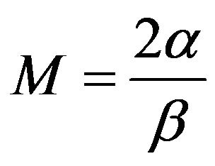
where M is a constant defined by twice the ratio between the two parameters, α and β and it is given as:
 (4)
(4)
 , is the minimum time associated with a constant value of the subcarrier
 (5)
(5)
with  represents the ceiling operator and
 is the chip spacing of the PRN code used in GNSS signals, given by the ratio between Coarse Acquisition
  GPS code chip spacing
  and the parameter
 .
.
The peak location of the CF can be accomplished by determining the position of the zero-crossing of the DC. Here, Early-minus-late correlators are necessary to determine the location of this zero-crossing. The early and late CFs in the traditional DLL scheme together with the DC for BOC (α, α) code, in coherent configuration, are shown in Figure 2. In the absence of MP and noise, the DC of the DLL is given by the following equation:
 (6)
(6)
where:  and
and  are respectively the late and early CFs.
R is the CF between the received and the locally generated signals. ∆ is the Early-minus-late spacing.
As this DC is function of the Early-minus-late spacing, it is also function of BOC subcarrier parameters such as α and β. The Figure 3 shows the form of this DC for different values of α, for β = 1 and with a small value of
 .
.
As shown in this figure, we observe the presence of several segments with different non null slopes and other segments with zero slopes. All These segments are function of α, β and ∆. In reference [38], the authors have proposed a mathematical model which characterizes the DC. The latter model is function of τ (τ represents  in [38]) and it contains some typing errors. In [39] we have corrected this model. This last is therefore given as follows:
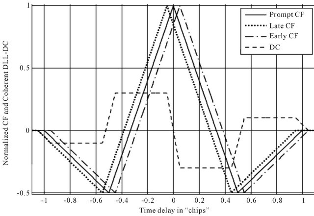
Figure 2. Construction of the DC of the DLL.
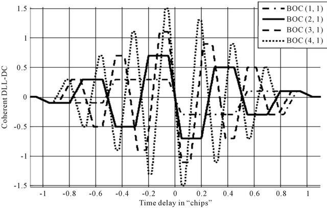
Figure 3. Normalized coherent DC for different values of α and β.
 (7)
(7)
with:
 (8)
(8)
 (9)
(9)
 (10)
(10)
 (11)
(11)
 (12)
(12)
In the non-coherent configuration, the normalized DC is given as follows [40]:
 (13)
(13)
The squared normalized CF can be given from Equation (3) as follows:
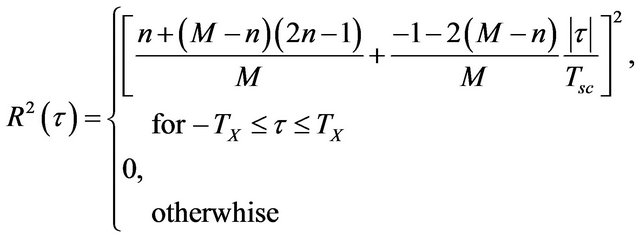 (14)
(14)
The Equation (13) can be simplified as follows:
 (15)
(15)
The non-coherent DC is function of the coherent one. Thus this equation can be simplified as follows:
 (16)
(16)
where:  is the coherent DC. The non-coherent DC is also function of α and β. The Figure 4 shows the form of this latter DC for different values of α and β and with the same value of Early-minus-late spacing.
The comparison between Figures 3 and 4 proves that in contrast to the coherent DLL-DC that have segments with different non-null slopes and others with zeros slopes, the non-coherent DLL-DC have both 1st order and 2nd order line segments.
The non-coherent DLL-DC can be calculated analytically segment by segment with the same geometrical method used in reference [38]. In fact, we define the different regions of non coherent DLL-DC as shown in Figure 5. This figure presents the general geometry associated with the non coherent DLL-DC.
As illustrated in this figure, the regions Di and  are numerated from −2M to 2M (i = −2M, −1, −2, ∙∙∙, 2M). Because the DLL-DC is an odd function, we calculate only the regions of
  and the remaining regions are obtained by symmetry.
All these regions can be derived geometrically from the Figure 5 and Equations (14) and (15) with the same formalism used in reference [38]. The difference between the model in [38] and our proposed one is the presence of both 1st and 2nd order equations in our proposed model instead of just the 1st order in [38].
Hence, these regions can be given as follows:
2.1. D0 Region
This region of duration , corresponding to “i = 0”, is unique and it is represented by a segment of positive slope which passes through the point (0, 0) and characterizes the first zero-crossing in the interval
 . indeed, it suffices to calculate the slope of this line segment for determining the corresponding function which is given as:
 (17)
(17)
After all calculations have been done, A0 can be calculated from Equations (14) and (15) and Figure 5 as follows:
 (18)
(18)
The interval of validity of this region can be given from Figure 5 as follows:
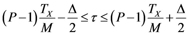
2.2. Di Regions for “i” Odd
These regions correspond to the odd values of “i”. They are represented by segments of 1st order and they have an interval of . The equations of these line segments are in the form:
 (19)
(19)
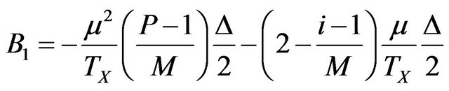
After all calculations have been done, A1 and B1 can be given as follows:
 (20)
(20)
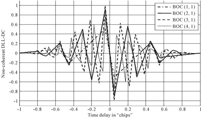
Figure 4. Normalized non-coherent-DC for different values of α and β.

Figure 5. Delimitation and notation of the various regions of the DLL curve of BOC (2, 1) code.
 (21)
(21)
The interval of validity of this region can be given from Figure 5 as follows:
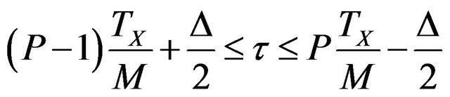
with: 
 (22)
(22)
2.3. Di Segments for “i” Even
These regions correspond to the even values of “i”. They are represented by segments of 2nd order. The equations of these 2nd order segments are in the form:
 (23)
(23)
A2, B2 and C2 can be calculated from Equations (14) and (15) and from Figure 5; they are given as follows:
 (24)
(24)
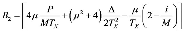 (25)
(25)
 (26)
(26)
The interval of validity of this region can be given from Figure 5 as follows:
 (27)
(27)
with: .
.
2.4. DM Segment
There exists another special case of non-coherent DLLDC for i = M in the interval . This case is unique and it represents the last segment of the non-coherent DLL-DC. It represents also the last segment of squared CF. This segment can be given from Equation (15) as follows:
 (28)
(28)
The general mathematical model corresponding to BOC (α, β) can be given as follows:
 (29)
(29)
with:
 (30)
(30)
 and
and .
.
3. Proposed Non-Coherent MP Tracking Error
MP propagation represents an important error source in GNSS positioning. This error is due to the fact that the signal reaches the receiver antenna by two or more paths. In urban environment the causes of MP include reflection from objects such as buildings. In presence of both LOS and one specular reflected signals, the baseband signal model is defined as follows [3]:
 (31)
(31)
with:
 : Delay of Line Of Sight (LOS) signal;
 : Delay of MP signal;
 : LOS signal amplitude;
 : MP signal amplitude;
 : Phase of LOS signal;
 : Phase shift due to the MP signal;
 : Additive White Gaussian Noise (AWGN);
 : PN code plus subcarrier.
Consequently, the receiver tries to correlate with all components of the received signal. Analytically, the LOS and MP signal may be treated separately. Thus, one may consider the CF associated with LOS (LOSCF) and the CF associated with MP signal (MCF). At any point, these two functions can be vector summed to yield the CF associated with the composite signal (CCF).
The normalized CF (with respect to ,
,  and
and ) of the composite signal can be given as [20]:
 (32)
(32)
with: : Ideal CF.
The CF of the received signal is distorted as shown in Figure 6 for BOC (α, α) code (Solid line).
Consequently, the distorted DLL-DC has a zerocrossing at non-zero code tracking error.
As shown in Figure 7, this distortion ensues in a shift between the received signal and the locally generated code provoking an error in the tracking process. In what follows we propose a general model of MP tracking errors of non-coherent DLL DC.
In the presence of MP signal the coherent DLL-DC is given as follows:
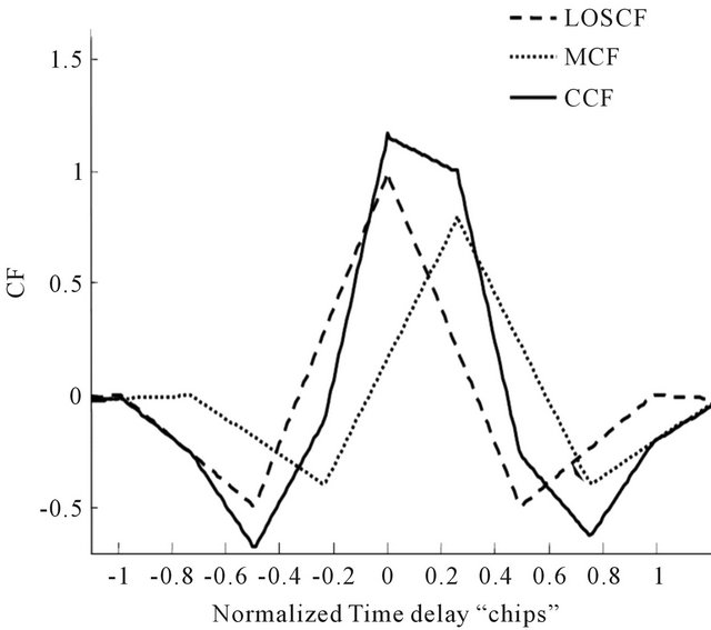
Figure 6. LOSCF, MCF and CCF of the BOC (α, α) code.
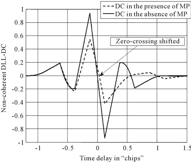
Figure 7. Non-coherent DLL-DC in the presence of MP.
 (33)
(33)
 (34)
(34)
Finally Equation (1) becomes:
 (35)
(35)
where  is the ideal coherent DLL-DC and:
 (36)
(36)
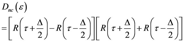
In the presence of MP signal the non-coherent DLLDC can be given as:
 (37)
(37)
Equation (37) becomes:
 (38)
(38)
 (39)
(39)
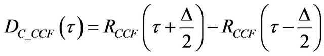
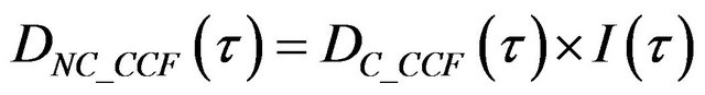
where:  is an error term given as:
 (40)
(40)
In contrast to the coherent discriminator that contains two terms characterizing respectively the LOS and the MP DCs (Equation (35)), the non-coherent DLL discriminator contains three terms (Equation (39)). In fact, the first term characterizes the non-coherent LOS DC, the second one characterizes the non-coherent MP DC and finally the third one characterizes the influence of the LOS on the MP and vice versa. To compute the noncoherent MP tracking error, we have to resolve the Equation (39) according to . The direct resolution of this equation presents a certain difficulty in comparison to the coherent configuration. In fact, a simplified form of this equation can be given as follows:

 (41)
(41)
 (42)
(42)
 (43)
(43)
where:
 (44)
(44)
According to this equation, we can conclude that the non-coherent DLL is function of the coherent one. In fact, the zero crossing of the non-coherent DLL is the same as that of the coherent one. This is because in the term of error, in Equation (40), which is clearly the sum of four CFs (Early-minus-late LOS CFs and Early-minus-late MP CFs), each Early-minus-late couple consists of two overlapping CFs whose sum is constant and non null in the linear zone  of the DC. This is explained by the equal but reversed slopes of their line segments in this interval. This constant is given as follows:
 for
for  (45)
(45)
The error term, the coherent DLL-DC and the product which characterizes the non-coherent DLL-DC for BOC (α, 1) LOS signal (α = 1, 2, 3 and 4) are illustrated in Figure 8.
As depicted in this figure, we first observe clearly that the term of error is constant and non null in the region of DC linear zone and thus it has an effect only on the variation of the slope of the non-coherent DLL-DC. In addition, the unique zero-crossing in this region is the one of the coherent DC. Consequently, non-coherent DLL tracking error is like that of the coherent one and it can be computed by solving the Equation (39). Thus, with the same mechanism used in reference [38], we can get the non-coherent MP tracking error as follows:
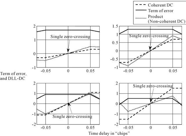
Figure 8. The term of error, the coherent DLL-DC and non-coherent DLL-DC for BOC (α, 1) LOS signal (α = 1, 2, 3 and 4).
 (46)
(46)
with
 (47)
(47)
 (48)
(48)
 (49)
(49)
 (50)
(50)
4. Test of the Proposed Closed form Solutions
Computer implementations have been performed to test the proposed models. In fact, NC structure, based on the block diagram of Figure 9, has been simulated using Matlab implementation to produce the numerical models. Thus, early late spacing ∆ is chosen equal respectively to
 ,
,  ,
,  and
and . The analytical models have been obtained by the implementation of Equations (29) and (46) in the same work-space (Matlab) for the same values of ∆.
Firstly we test the non-coherent DLL-DC model. In fact, we present the case of LOS signal without MP signal. The DCs of both analytical and numerical models are shown in the Figures 10-12 for different BOC (α, β) modulated signals.
As shown in all these figures the proposed analytical
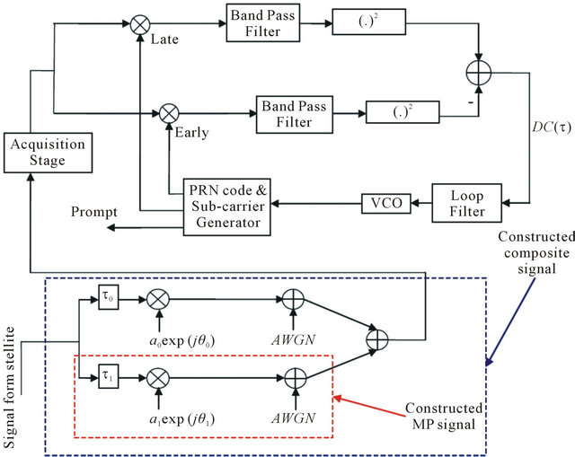
Figure 9. Non-coherent DLL in presence of MP.
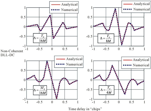
Figure 10. Comparison of proposed and numerical models of normalized DC for BOC (1, 1) code.
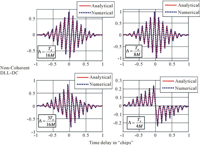
Figure 11. Comparison of proposed and numerical models of normalized DC for BOC (6, 1) code.
models coincide with the numerical ones.
Secondly we test the non-coherent MP tracking error. In fact, we present the case of LOS and MP signals where the infinite bandwidth filter in the receiver has been considered. The MP has an amplitude that is equal to 0.5 with respect to the LOS. The MP delay is varied from 0 to TX in meters with respect to the LOS. The phase of the MP is taken equal to 0˚ and 180˚ with respect to the LOS (These values correspond to the maximum MP tracking error). The MP and the composite signals are constructed based on the diagram of Figure 9. The non-coherent MP tracking errors are shown in Figures 13-15 for respectively BOC (1, 1), BOC (6, 1) and BOC (15, 10).
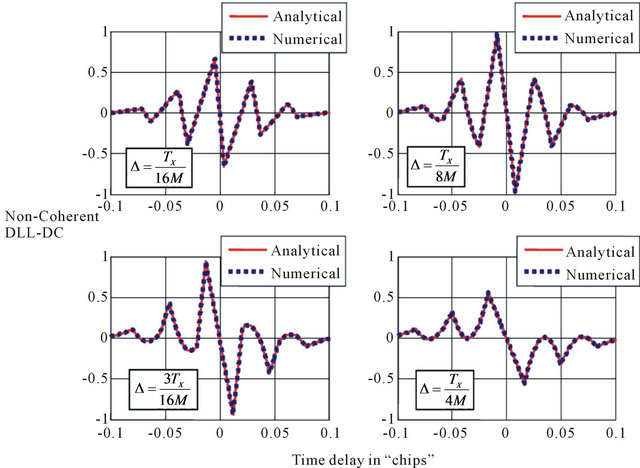
Figure 12. Comparison of proposed and numerical models of normalized DC for BOC (15, 10) code.
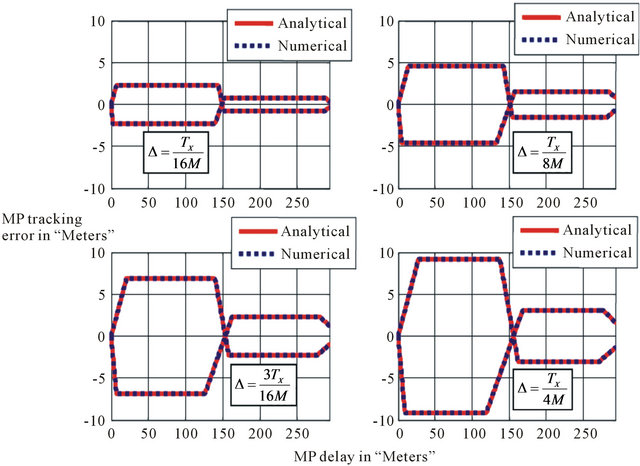
Figure 13. Comparison of proposed and numerical models of envelope offset error of BOC (1, 1) code.
As illustrated in all these figures the proposed noncoherent tracking errors models coincide with the numerical ones showing the efficiency of the proposed models.
5. Conclusion
In this paper, analytical models of non-coherent DLLDCs and MP tracking error envelopes have been proposed. The models development is more complex with regard to that of the coherent one. In fact, contrary to the coherent DC models that contain line segment of first order, the non-coherent ones contain segments of both first and second order. Also we have developed the noncoherent MP tracking error envelopes and we have illus-

Figure 14. Comparison of proposed and numerical models of envelope offset error of BOC (6, 1) code.
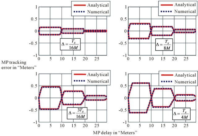
Figure 15. Comparison of proposed and numerical models of envelope offset error of BOC (15, 10) code.
trated that they are similar to the coherent ones. The proposed models are valid for all BOC (α, β) modulated signals. The computer implementations have shown that the proposed analytical models coincide with the numerical ones which illustrate the efficiency of the proposed models.