A Gibbs Sampling Algorithm to Estimate the Parameters of a Volatility Model: An Application to Ozone Data ()
1. Introduction
We are going to split this section into two parts. One containing a general literature review and another focussing on the description of what happens in Mexico City.
1.1. General Literature Review
It is a well know fact that when exposed to high levels of pollution, human beings may present serious health issues (see for instance [1-3]). In particular, if ozone concentration levels stay above 0.11 parts per million (0.11 ppm) for a long period of time, then a very sensitive part of the population may present a deterioration in their health (see for instance [4-7]).
Since exposure to high levels of pollution can cause serious damage to people’s health as well as the environment in general, there are several works in the literature that deal with the problem of modelling the behaviour of pollutants in general and in particular, ozone. Among them, we may quote the early work [8] considering extreme value theory. We also have [9] using time series analysis; [10] and [11] considering Markov chain models; [12] with an analysis of the behaviour the maximum measurements of ozone with an application to the data from Mexico City; [13,14] using homogeneous Poisson processes, and [15,16] using non-homogeneous Poisson processes (for several Markov and Poisson models applied to air pollution problems see for instance
[17]). [18-20] present studies that analyse the impact on air quality of the driving restriction imposed in Mexico City.
Besides keeping track of the level of the daily maximum concentration of a pollutant and checking for a decreasing trend in the measurements, it might also be of importance for the environmental authorities to keep track of the degree of variability of the pollutant’s concentration. That is important because, for instance, it may help to see how the variability behaves after some measures aiming to reduce its level are taken. A decreasing of the daily concentration might occur, but it is also interesting to know if the variability also decreases. Following in that direction we have, for instance, [21,22] and [23] where some univariate and bivariate stochastic volatility models are used to study the weekly averaged ozone concentration in Mexico City. Also, in [23] and [24] we have the use of multivariate stochastic volatility models to study the behaviour of five pollutants present in the city of São Paulo, Brazil.
Many more works may be found in the literature. Some of those works consider spatial models and neural networks, among other methodologies. Some of them consider different pollutants as well. In this work we are going to consider only ozone since this pollutant is the one still causing problems in Mexico City. In the next section we describe the situation in Mexico City, the problem to be studied as well as the methodology considered to study it.
1.2. Description of the Problem in Mexico City
During the past twenty five years, environmental authorities in Mexico have been implementing several measures in order to decrease the level of pollution in several cities throughout the country. In particular, in Mexico City, those measures have caused an improvement in the air quality. For instance, from 1997 to 2005 the maximum hourly ozone measurements decreased by 30%. Moreover, during the period of time ranging from 2008 to 2010, the mean concentration of the daily maximum measurements did not surpassed the value 0.1 ppm. Taking into account that the Mexican environmental standard for ozone is 0.11 ppm ([25]) and individuals should not be exposed, on average for a period of one hour or more once a year, this value for the mean is not so bad. However, that does not mean that high levels do not occur. In order to see that, note that during the period from 01 January 2008 to 31 December 2010, there were 491 days with the daily maximum measurement surpassing the value 0.11 ppm, 22 days when the threshold 0.17 ppm was surpassed, and one day of surpassings of the threshold of 0.2ppm used to declare emergency alerts in Mexico City.
Figure 1 shows the plots of the daily maximum ozone measurements obtained during the period ranging from 01 January 2008 to 31 December 2010. The horizontal line indicates the Mexican ozone standard of 0.11 ppm.
Looking at Figure 1, we may see that even though the mean of the measurements in all regions is below 0.11 ppm, we may still have many days in which the daily maximum measurement is well above 0.11.
As seen in Figure 1, it would be useful to analyse how the ozone measurements variability have behaved in more recent years. In here we are analysing this variability. Once we are able to model it we will able to estimate the frequency at which emergency situations may occur. In the present paper, in order to analyse the behaviour of this variability, we also consider stochastic volatility models to analyse the ozone data set collected from the monitoring network of the Metropolitan Area of Mexico City (www.sma.df.gov.mx/simat/) corresponding to three years of the daily maximum ozone measurements. The advantage of using stochastic volatility models to analyse time series is that they assume the existence of two processes modelling the series. One modelling the observations and another modelling the latent volatility.
The model considered here is a particular case of the multivariate case considered in [23] and [24]. The difference here is that instead of using five pollutants we are going to concentrate only on ozone measurements obtained in five regions of Mexico City. Another difference is that in previous works, estimation of the parameters of the model was performed using the Gibbs sampling algorithm internally implemented in the software WinBugs ([26]). That poses some difficulties such as slow con-

Figure 1. Daily maximum ozone measurements for regions NE, NW, CE, SE and SW for the period ranging from 01 January 2008 to 31 December 2010.
vergence of the algorithm and the use of very specific and very informative prior distributions. That was responsible for the need of running the algorithm several times until the right values for the hyperparameters were obtained. In here, the Gibbs sampling algorithm is programmed in R. The convergence was attained more rapidly and the prior distributions, even though informative, were not so difficult to adjust. Hence, another aim here is to present the Gibbs sampling algorithm, and its code, used to estimate the parameters of the stochastic volatility model and apply it to the case of ozone data from Mexico City.
This paper is organised as follows. Section 2 presents the stochastic volatility model considered here as well as the vector of parameters that need to be estimated. A Bayesian formulation used to estimate the parameters of the model considered in Section 2 is given in Section 3. In Section 4 the model and parameters estimation described in Sections 2 and 3 are applied to the data set obtained from the monitoring network of Mexico City. Section 5 presents some remarks and discussion of the results obtained. Finally, in Section 6 we conclude. An Appendix with the computer code used in the estimation of the parameters of the model is given after the list of reference.
2. A Stochastic Volatility Model
Stochastic volatility models have been used, in general, to analyse the variance of time series of financial returns (see for instance [27-30]). Until then, the existing methodology considered to model the volatility could be characterised by those used to model the variance based on function of past observations of the series (for instance the ARCH—auto regressive conditional heteroscedastic-models proposed by [31]) and of the delayed values of the series (GARCH—generalised auto regressive conditional heteroscedastic—models proposed by [32]). Volatility models are characterised by modelling the volatility of the times series in function of a non observable stochastic process. Hence, the main difference between the two approaches is that models based on GARCH assume that the volatility is observed in a period ahead in time, while in the stochastic volatility models, the volatility is a latent variable that cannot be observed without an error.
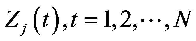
In this section the stochastic volatility model used to study the behaviour of weekly average measurements of the ozone in several regions of Mexico City is described. Many types of multivariate stochastic volatility models may be found in the literature (see for example [30]). The one considered here may be described as follows. Let  and
and  be fixed known integer and real numbers, respectively. (In here, N will represent the number of weeks in the observational period
  whose weekly average measurements of ozone we are considering.) Also, let
  be an integer number recording the number of different regions where measurements are taken. Hence, for
 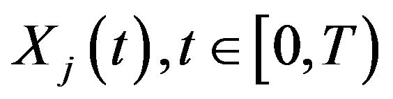 the daily maximum ozone concentration measured on region
  on the tth day,
  , define
 by
by 
 , and so on. Therefore,
  is the weekly averaged ozone concentration in region
  in the tth week,
 .
.
Denote by  the log-return series defined by
 . Let
. Let
 be a K-dimensional vector whose coordinates are the
  times series
 . The vector
  is known as the log-return vector of the series
 . The set
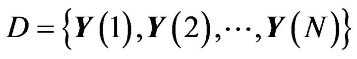 will denote the set of observed data.
As in [23] and [24], we assume that  may be written as
 , where
 is an error vector and
 is a
is a  diagonal matrix given by
 , with
 a vector of latent variables to be specified later. Therefore, we may write
 , as
, as .
.
Also, we assume that  is such that its coordinates follow an AR(1) model, i.e., for

where , and
, and  is assumed to have a multivariate Normal distribution with mean vector
  and variance-covariance matrix
  the diagonal matrix
 .
.
Remark. Note that by definition we have, for  , that
  has a Normal distribution
 and that given
 , the variable
 has a Normal distribution
 .
.
We also assume that  has a multivariate Normal distribution with mean vector
  and variance-covariance matrix
 , where
 is the variance of
 , and
, and  is the covariance of
  and
and 
 . Therefore, by definition, we have that given
 , the vector
  has a multivariate Normal distribution with mean vector 0 and variance-covariance matrix given by
 , where
  and
and .
.
Remark. Note that since the volatility of the series , is by definition
 , the vector
 is the vector of the logarithm of the volatility of the series studied.
In the present work we will be considering the case where  i.e., we assume independence among the coordinates of the vector
 . Hence, now
 . That is, we are considering only Model I given in [24]. This means that the problem can be viewed as having
  times series which can be analysed separately.
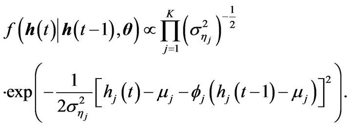
Therefore, the joint density function of  given
given  is
is
 (1)
(1)
This means that given , the vector of the log-returns
 has a Normal distribution with mean vector
  and variancecovariance matrix
 .
.
The vector of parameters to be estimated is
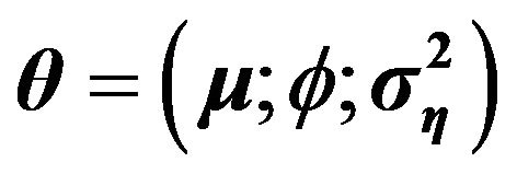 , where
 ,
,
 and
and . (In here,
  indicates the vector
  transposed.)
3. Bayesian Formulation of the Models
In this section the expression for the complete conditional marginal density functions of the parameters, that are used in the Gibbs sampling algorithm, are presented. We also determine the prior distribution of the parameters of the model. Therefore, define , where
 . The aim is to obtain an expression for the posterior distribution
  and from it obtain the estimated parameters. Note that we have that
 , where
  is the likelihood function of the model,
  and
and  are the conditional distribution of the latent variables given the vector of parameters and the prior distribution of the vector of parameters, respectively.
Note that the likelihood function  is given by
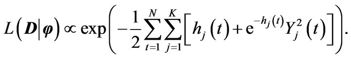 (2)
(2)
Additionally,

By hypothesis, we have that ([23] and [24])

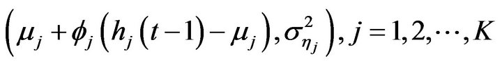
and that for ,
,
Hence,
 (3)
(3)
The choice of prior distributions for the parameters was based on information obtained from previous studies ([22-24]) and also from the behaviour presented by the data.
The parameters  will have as their prior distributions a Normal distribution Normal
 , a Normal
 and an inverse Gamma IG
 . The hyperparameters
 will be considered known and will be specified later. (In here, IG
 is the inverse Gamma distribution with mean
and variance .)
.)
The latent variables  will be considered as parameters to be estimated and will have as their prior distribution a Normal
  for
for , and for
 its prior distribution is a Normal
 .
.
Therefore, we have from (2), (3) and the forms of the prior distributions of the parameters, that the complete posterior distribution  is given by
 (4)
(4)
Due to the complexity of (4), estimation of the parameters of the volatility models may not be performed using usual methods. Hence, Markov chain Monte Carlo algorithms will be used. In particular, a Gibbs sampling algorithm (see for instance [33]) programmed using R is going to be used to obtain a sample of the parameters and with that estimates for them.
Therefore, we need the expression for the complete marginal conditional distribution for each parameter. Additionally, in some cases, in order to obtain a sample from those complete conditional marginal distributions, we will need to use a Metropolis-Hastings algorithm (see for instance [34-36]) step inside the Gibbs sampling. Therefore, whenever necessary, the acceptance probability for the Metropolis-Hastings algorithm is also going to be presented.
Hence, let  indicate the vector
  without the coordinate containing the parameter
 . Therefore, from (4) we have, for
 , that

where

and for ,
,
where
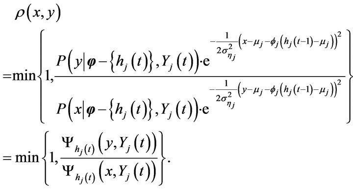
Therefore, in the case of , if
, if  is the new proposed value for
  and
and  is its actual value, then the acceptance probability in the MetropolisHastings step is given by (we use the respective prior distributions to generate the proposed values)

for  and for
 ,
,
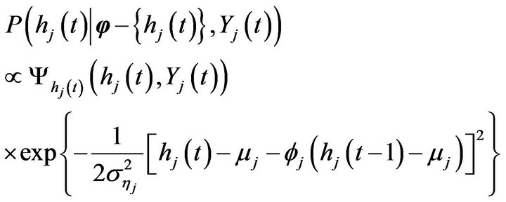
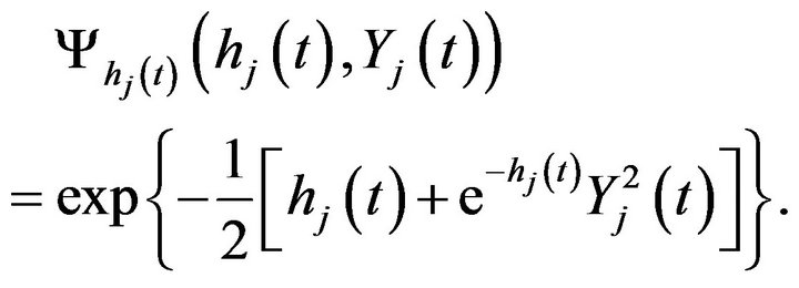
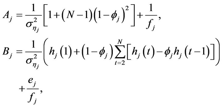
Additionally, we have, for , that
 is proportional to a Normal
 , where
that  is proportional to a Normal
 , with

and that  is proportional to a inverse Gamma IG
 where
where

Convergence of the Gibbs sampling algorithm was monitored using the analysis of the trace plots and the package CODA that is part of the software R. Specifically, we used the Geweke ([37]), Raftery-Lewis ([38]), Heidelberger-Welch ([39]) and the Gelman-Rubin ([40]) tests.
4. An Application to Mexico City Ozone Measurement
In this section we apply the stochastic volatility model, described in earlier sections, to ozone measurements from the monitoring network of Mexico City. The Metropolitan Area of Mexico City is divided into five sections, namely, NE (Northeast), NW (Northwest), CE (Centre), SE (Southeast) and SW (Southwest) (see for instance [10], [15] and http://www.sma.df.gob.mx). The data used here correspond to the daily maximum ozone measurements taken from 01 January 2008 until 31 December 2010, corresponding to  observations. Measurements are taken minute by minute and the 1-hour average results is reported at each monitoring station. The daily maximum measurement for a given region is the maximum over all the maximum averaged values recorded hourly during a 24-hour period by each station placed in the region. During the period of time considered, the mean concentration levels for regions NE, NW, CE, SE and SW are, respectively, 0.0829, 0.0851, 0.0876, 0.0911, and 0.0977 with respective standard deviation given by 0.0286, 0.0303, 0.0306, 0.0294 and 0.0341. We also have a total of
  weeks and note that in here
 . We associate k = 1, 2, 3, 4 and 5, with regions NE, NW, CE, SE and SW, respectively.
Figure 2 presents the plots of the weekly averaged measurements for each of the regions during the period of time considered here.
Note that the weekly averaged measurements also present low values in a large number of weeks. However, it seems that the variation from one week to another may, in some cases, be very high. Therefore, it is of interest to know how this variability is behaving. Using stochastic volatility models we will be able to obtain information on how the variation behaves and with the estimated values
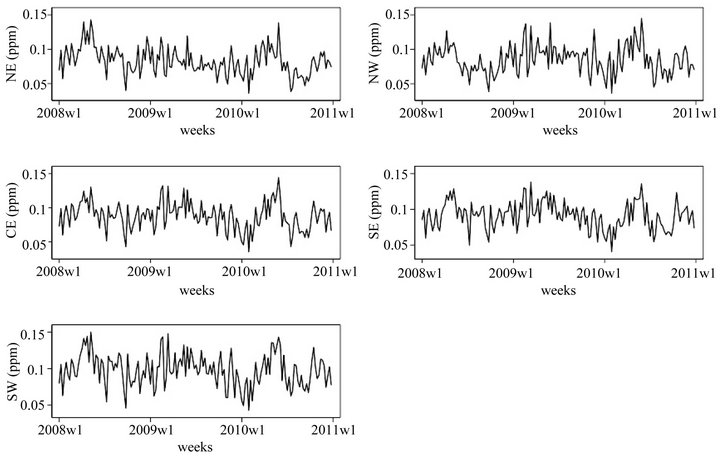
Figure 2. Weekly averaged ozone measurements for regions NE, NW, CE, SE and SW for the period ranging from 01 January 2008 to 31 December 2010.
of the parameters of the model, we may perform predictions about future behaviour of this variability. As said before, estimation of the parameters is going to be made using a sample from the respective complete conditional marginal posterior distributions which will be drawn using the Gibbs sampling algorithm run for three separate chains. Each chain run 21000 steps and after a burn-in period of 2000 steps, a sample of size 3800, taken every 5th generated value, was obtained from each one. Hence, estimation of the parameters was performed using a sample of size 11400. The hyperparameters of the prior distributions are aj = 0, bj = 1, cj = 3, dj = 3, ej = 0, fj = 10, j = 1, 2, 3, 4, 5. Table 1 presents the mean, the standard deviation (indicated by SD) and the 95% credible intervals for the parameters of the model when data from each of the regions are used.
In Figures 3-5, we have the plots of the estimated (dashed lines) and observed (solid lines) log-returns of the weekly averaged measurements for the entire observational period and including the predicted and the observed values for the month of January 2011 (not included in the data when estimating the parameters).
Observing Figures 3-5, we may see that, most of the time, the estimated log-returns of the weekly averaged measurements provide a good fit to the observed ones.

Table 1. Posterior mean, standard deviation (indicated by SD) and 95% credible intervals of the parameters of interest for all regions.


Figure 3. Observed (solid line) and estimated/predicted (dashed) log-returns of the weekly averaged measurements for regions NE and NW for the period ranging from 01 January 2008 to 31 December 2010/31 January 2011.


Figure 4. Observed (solid line) and estimated/predicted (dashed) log-returns of the weekly averaged measurements for regions SE and SW for the period ranging from 01 January 2008 to 31 December 2010/31 January 2011.

Figure 5. Observed (solid line) and estimated/predicted (dashed) log-returns of the weekly averaged measurements for region CE for the period ranging from 01 January 2008 to 31 December 2010/31 January 2011.
5. Discussion
In this paper we have considered a particular version of a multivariate stochastic volatility model to study the behaviour of the weekly ozone averaged measurements. The interest was in the variability of the series of measurements. The parameters present in the model were estimated using a Gibbs sampling algorithm. This algorithm was implemented using the package R and the code is given in the Appendix of this work. Even though the model considered here is a particular case of a more general version, the general approach may also be implemented by making some adjustments in the code.
Looking at Table 1, we may see that the values of the parameters are very similar in all regions. That is justified by the fact that the weekly averaged measurements behave in a very similar way in all regions during the observational period (see Figure 2). Hence, the logreturns series will reflect that behaviour. Also from Table 1, we may see that the effect of the parameter  on the latent variables is a negative one in all regions. That effect is also observed in similar studies ([22,23]). Note that in all regions the value of
  is very small. That means that the effect of past values in the present ones is very small. That same behaviour is also seen in [22,23]. However, for the present dataset the effect is even smaller.
Using the estimated parameters given in Table 1, we may obtain estimates for the averaged weekly measurements in future weeks. In order to illustrate that we consider the month of January 2011. Note that, by hypothesis we have, for each , that
 , and therefore, we may write
 , where
 . Hence, using the value of the last week of December 2010 (which would be
 ), and using the simulated values for
  and
and  we may obtain an estimate for the averaged measurement of the first week of January 2011. This values is used as
  in the next step. Again, we simulate values for
  and
and  and with that we obtain the new
 , which will correspond to the second week of January 2011, and so on. Those estimated values and the observed ones are given in Table 2.
Looking at Table 2 we may observe that for the first two weeks of January 2011 the estimated weekly averaged values overestimate the observed ones. However, for the last two weeks, the observed weekly averaged measurements are underestimated. The error in the estimation may be justified by the accumulated errors that might occur during the estimation of  and
and . Nevertheless, the approximation is overall very good. That can also be corroborated by looking at the plots of the log-returns given in Figures 3-5.
6. Conclusions
Even though the version of the model considered here assume independence among regions, it is possible to see, by looking at Figures 3-5 and at Table 2, that the
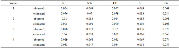
Table 2. Observed and predicted weekly averages ozone measurements for the month of January 2011.
estimated quantities provide a good approximation to the observed one as well as providing a good prediction to future observations.
Since it provides an instrument to be used to estimate the parameters in volatility models, the programme code given in this work may help those interested in studying volatility of times series in general. Even though the model is applied to air pollution data, the code may be used in any dataset.
We would like to call attention to the fact that a model where correlation amongst the regions is considered may provide a better insight on the behaviour of the volatility of the weekly averaged measurements. That would incorporate the possible effect that the wind direction may have on the measurements in different regions. In the present work we have not dealt with that, but as mentioned before a modification on the complete conditional marginal posterior distributions and on the code of the programme can be easily made in order to incorporate those cases. However, that is the subject of future studies.
7. Acknowledgements
The authors would like to thank an anonymous reviewer for the comments that helped to improve the presentation of this work. Financial support was received from the Dirección General de Apoyo al Personal Académico of the Universidad Nacional Autónoma de México through the project PAPIIT number IN104110-3 and is part of VDJR’s MSc. Dissertation.
Appendix
# GIBBS SAMPLING ALGORITHM
# Auxiliary functions psi_hj1=function(hj1,yj1){
b_2=exp(-1/2*(hj1+exp(-hj1)*yj1^2))
b_2
}
#####################################
psi_hjt=function(hjt,yjt){
b_1=exp(-1/2*(hjt+exp(-hjt)*yjt^2))
b_1
}
#####################################
# Initial data n=21000 burn=2000 n.cadenas=3 salto=5 region=1 seed=987 if(seed>0){set.seed(seed)}
a1=0 ;b1=1 c1=3 ;d1=3 e1=0 ;f1=10
# Generating the initial values in_mu=rnorm(n.cadenas,0,1)
in_phi=rnorm(n.cadenas,0,0.35)
in_sigma2=1/rgamma(n.cadenas,3,2)
######################################
mide.tiempo=proc.time()
if(region==1){y1=scan("c:/r/rsne3.txt")}
if(region==2){y1=scan("c:/r/rsnw3.txt")}
if(region==3){y1=scan("c:/r/rsce3.txt")}
if(region==4){y1=scan("c:/r/rsse3.txt")}
if(region==5){y1=scan("c:/r/rssw3.txt")}
N=155 # number of weeks (three years)
espmu=e1;espphi=a1;espsigma2=d1/(c1-1)
######################################
# Storing the values of the chains SIMmu=matrix(0,n,n.cadenas)
SIMphi=matrix(0,n,n.cadenas)
SIMsigma2=matrix(0,n,n.cadenas)
Hjtn=matrix(0,n,N*n.cadenas) # store simulated value of
# h Contador=matrix(0,N,n.cadenas) # store accepted Metro# polis-Hasting values
#####################################
for(m in 1:n.cadenas){
######################################
# Gibbs simulation of the latent variables (n=1)
# h_j, t=1,2,...,155; N=155
# First step for t=1
# Metropolis-Hastings step in the Gibbs sampling anterior=in_mu[m] # initial value for h_j(1)
u=runif(1)
y=rnorm(1,in_mu[m],sqrt(in_sigma2[m])) # proposal
# density num=psi_hj1(y,y1[1])
den=psi_hj1(anterior,y1[1])
rho=num/den Hjtn[1,(N*(m-1)+1)]=anterior+(y-anterior)*(u<=rho) #
# first simulated Gibbs value Contador[1,m]=(u<=rho)
# simulation for t=2,3,...,N for(t in 2:N){
hj_ant=Hjtn[1,(N*(m-1)+t-1)] # Gibbs actualization anterior=rnorm(1,hj_ant,sqrt(in_sigma2[m])) # initial
# value u=runif(1)
y=rnorm(1,in_mu[m]+in_phi[m]*(hj_ant-in_mu[m]),sqrt(in_sigma2[m])) # proposed value num=psi_hjt(y,y1[t])
den=psi_hjt(anterior,y1[t])
rho=num/den Hjtn[1,(N*(m-1)+t)]=anterior+(y-anterior)*(u<=rho)
Contador[t,m]=(u<=rho)
}
###################################
# mu_1--->n=1
# Gibbs actualisation
# h_1=Hjtn[1,(N*(m-1)+1):(N*(m-1)+N)]
# Gibbs actualisation#
# Parameters of the complete conditional marginal densi# ties
##########
A=1/f1+(1+(1-in_phi[m])^2*(N-1))/in_sigma2[m]
diferencias=numeric(N)
for(t in 2:N){
diferencias[t]=h_1[t]-in_phi[m]*h_1[t-1]}
B=e1/f1+(h_1[1]+(1-in_phi[m])*sum(diferencias))/in_sigma2[m]
C=B/A; D=1/A
################################################
SIMmu[1,m]=rnorm(1,C,sqrt(D))
###################################
# phi_11--->n=1
# Gibbs actualisation#
mu_1=SIMmu[1,m]
#Gibbs actualisation#
#Parameters of the complete conditional marginal densi# ties
##########
diferencias1=numeric(N)
for(t in 2:N){
diferencias1[t]=(h_1[t-1]-mu_1)^2}
A=1/b1+sum(diferencias1)/in_sigma2[m]
diferencias2=numeric(N)
for(t in 2:N){
diferencias2[t]=(h_1[t]-mu_1)*(h_1[t-1]-mu_1)}
B=a1/b1+sum(diferencias2)/in_sigma2[m]
C=B/A; D=1/A
################################################
SIMphi[1,m]=rnorm(1,C,sqrt(D))
###################################
# sigma2_1--->n=1
# Gibbs actualisation#
phi_1=SIMphi[1,m]
# Gibbs actualisation#
# Parameters of the complete conditional marginal densi# ties
##########
A=c1+N/2 diferencias=numeric(N)
for(t in 2:N){
diferencias[t]=(h_1[t]-mu_1-phi_1*(h_1[t-1]-mu_1))^2}
B=1/2*((h_1[1]-mu_1)^2+sum(diferencias))+d1
################################################
SIMsigma2[1,m]=1/rgamma(1,A,B)
##########################################
# Gibbs simulation for n=2,3,...##########################################
for(k in 2:n){
# Gibbs actualisation#
mu_1=SIMmu[k-1,m]
phi_1=SIMphi[k-1,m]
sigma2_1=SIMsigma2[k-1,m]
# Gibbs actualisation#
# h_j, t=1 anterior=Hjtn[k-1,(N*(m-1)+1)]
u=runif(1)
y=rnorm(1,mu_1,sqrt(sigma2_1))
num=psi_hj1(y,y1[1])
den=psi_hj1(anterior,y1[1])
rho=num/den Hjtn[k,(N*(m-1)+1)]=anterior+(y-anterior)*(u<=rho)
Contador[1,m]=Contador[1,m]+(u<=rho)
# simulating h_j, t=2,3,...,N for(t in 2:N){
hj_ant=Hjtn[k,(N*(m-1)+t-1)]
anterior=Hjtn[k-1,(N*(m-1)+t)]
u=runif(1)
y=rnorm(1,mu_1+phi_1*(hj_ant-mu_1),sqrt(sigma2_1))
num=psi_hjt(y,y1[t])
den=psi_hjt(anterior,y1[t])
rho=num/den Hjtn[k,(N*(m-1)+t)]=anterior+(y-anterior)*(u<=rho)
Contador[t,m]=Contador[t,m]+(u<=rho)
}
###################################
# mu_1-->>n=k
# Gibbs actualisation#
h_1=Hjtn[k,(N*(m-1)+1):(N*(m-1)+N)]
# Gibbs actualisation#
# Parameters of the complete conditional marginal densi- # ties
##########
A=1/f1+(1+(1-phi_1)^2*(N-1))/sigma2_1 diferencias=numeric(N)
for(t in 2:N){
diferencias[t]=h_1[t]-phi_1*h_1[t-1]}
B=e1/f1+(h_1[1]+(1-phi_1)*sum(diferencias))/sigma2_1 C=B/A; D=1/A
################################################
SIMmu[k,m]=rnorm(1,C,sqrt(D))
###################################
# phi_11-->>n=k
# Gibbs actualisation#
mu_1=SIMmu[k,m]
# Gibbs actualisation#
#Parameters of the complete conditional marginal densities
##########
diferencias1=numeric(N)
for(t in 2:N){
diferencias1[t]=(h_1[t-1]-mu_1)^2}
A=1/b1+sum(diferencias1)/sigma2_1 diferencias2=numeric(N)
for(t in 2:N){
diferencias2[t]=(h_1[t]-mu_1)*(h_1[t-1]-mu_1)}
B=a1/b1+sum(diferencias2)/sigma2_1 C=B/A; D=1/A
################################################
SIMphi[k,m]=rnorm(1,C,sqrt(D))
###################################
# sigma2_1-->>n=k
# Gibbs actualisation#
phi_1=SIMphi[k,m]
# Gibbs actualisation#
# Parameters of the complete conditional marginal densi# ties
##########
A=c1+N/2 diferencias=numeric(N)
for(t in 2:N){
diferencias[t]=(h_1[t]-mu_1-phi_1*(h_1[t-1]-mu_1))^2}
B=1/2*((h_1[1]-mu_1)^2+sum(diferencias))+d1
################################################
SIMsigma2[k,m]=1/rgamma(1,A,B)
}}
NOTES