Large and Moderate Deviations for Projective Systems and Projective Limits ()
1. Notation and Basic Results
Definition 1.1. Let E be a Hausdorff topological space, F a σ-algebra of subsets of E, and  (with D a directed set) a net of probability measures (p.m.’s) defined on F. We say that, the net of p.m.’s
  satisfies the full large deviations principle ([1,2]), with normalizeing constants
  (
( such that
 ) and rate function
 , if I is lower semi-continuous and
 , we have:
1) (upper bound)
 (1)
(1)
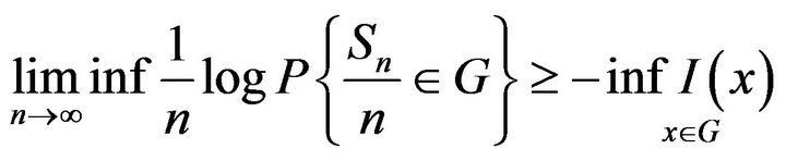
2) (lower bound)
 (2)
(2)
with cl(B) (int(B)) the closure (respectively the interior) of the set Β.
If, in addition,  (level set) is compact, I is called a good rate function.
Remark 1.2.
If the upper bound is valid for all compact sets, while the lower bound is still true for all open sets, we say that the net of p.m.’s  satisfies the weak large deviations principle.
In order to “pass” from a weak LDP to a full LDP we have to find a way of showing that, most of the probability mass (at least on an exponential scale) is concentrated on compact sets. The tool for doing this, is the following.
Definition 1.3.
A net of p.m.’s  defined on (E,F) is called exponentially tight, if
  there is a compact set
  (subset of E) such that:
 (3)
(3)
Exponential tightness is applied to the following proposition to strengthen a weak large deviations result. A proof of the proposition can be found in [1].
Proposition 1.4.
Let  be a net of p.m.’s defined on
  that is exponentially tight.
Then: a) if the upper bound holds for all compact sets, then it also holds for all closed sets.
b) if the lower bound holds for all open sets, then the rate function is good.
Now, we will characterize families of topological spaces. This special kind of families will play an important role in proving large deviations results.
Definition 1.5. The family , with A a directed set, is called a projective system if:
1)  is a Hausdorff topological space 2)
  is a continuous, subjective map such that, if:
  Also,
Also,  is the identity map on
 .
.
We also consider a Hausdorff topological space E, F a σ-algebra of subsets of E and  a continuous, surjective map s.t. if
and for then
then .
.
The following two theorems give large deviations results in the case of projective systems [3].
Theorem 1.6. Let E be a Hausdorff topological space, F a σ-algebra of subsets of E s.t.: a) F contains the class of compact sets and b) F contains a base U for the topology.
Let  be a projective system and
 be as above. Assume that
  is measurable when E is endowed with F and
  with the Borel σ-algebra. Let
  be a net of p.m.’s on F and assume that:
i) , the net of p.m.’s
  satisfies a large deviations principle with normalizing constants
  and rate function

ii) the net of p.m.’s  is exponentially tight.
Then, the net  satisfies the large deviations principle with normalizing constants
  and good rate function
 .
.
When E is endowed with a specific topology (namely the topology induced by the maps ), Theorem 1.6 has the following form.
Theorem 1.7. Let E,  be as in theorem 1.6. Endow E with the initial topology induced by the maps
  and let F be the σ-algebra of subsets of E such that
  is measurable, where
  is endowed with its Borel σ-algebra
 . Let
. Let  be a net of p.m.’s on F and assume that:
i) , the net of p.m.’s
  satisfies a large deviation principle with normalizing constants
  and rate function
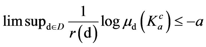
ii) there is a function  such that
 the set
 is compact and
 :
:

Then, the net of p.m.’s  satisfies the large deviations principle with normalizing constants
 and good rate function Ι, and
 .
.
On early days, large deviations results were proved using “large” spaces. One of these spaces is described below.
Definition 1.8. Let  be a projective system. The projective limit of this system (denoted by
 ) is the subset of the product space
  which consists of the elements
  for which
 when
when , endowed with the topology induced by Υ ([2]).
The following basic result, analogous to that of Theorem 1.7, allows one to transport a large deviations result on a “smaller” topological space to a “larger” one.
Theorem 1.9. Dawson-Gärtner (large deviations for projective limits).
Let  be a net of p.m.’s defined on
 . Assume that
 , the net of p.m.’s
  satisfies the full large deviations principle with constants
  and good rate function
 . Then, the net of p.m.’s
  satisfies the full large deviations principle with constants
  and good rate function:
 (4)
(4)
Remark 1.10. The space E of Theorem 1.9 is specificnamely  (in Theorem 1.7 E is arbitrary).
Theorem 1.9 is a special case of the Theorem 1.7.
Proof. (of Theorem 1.9)
Define the map . It is easy to see (using properties of the projective limits) that
 the map
 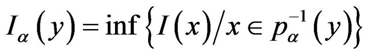 i.e.
i.e.
condition ii) of Theorem 1.7 is satisfied. Then, theorem 1.9 follows from Theorem 1.7.
The motivation for this paper was to find a “unified” way of proving large deviations results. This is done by using the projective systems approach. Using this approach, and not the one of projective limits, the proofs of most of the basic results of the theory are much easier and simpler, the arguments direct. Also, we are able to prove extensions of these results to more abstract spaces, at least in the case of exchangeable sequences of r.v.’s.
2. Applications
We now give some of the basic results of the large deviations theory. Extensions of these theorems can be easier proved using projective systems.
1) Theorem 2.1. (Cramer)
Let  be a sequence of independent and identically distributed (i.i.d) random variables (r.v.’s), taking values in
  with (common) distribution
and .
.
1) If
 (5)
(5)
then: a) (upper bound)  closed:
 (6)
(6)
with
and
 (7)
(7)
b) , the set
 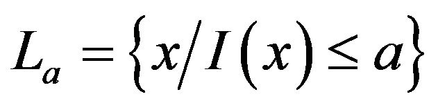 is compact.
2) (lower bound)  open:
open:
 (8)
(8)
Theorem 2.2 generalizes Cramer’s theorem in the case of a separable Banach space. The proof is given here using projective systems.
Theorem 2.2. (Donsker-Varadhan 1976) (Generalization of Cramer’s theorem)
Let E be a separable Banach space and F its Borel σ-algebra. Let  be a sequence of i.i.d. E-valued r.v.’s and
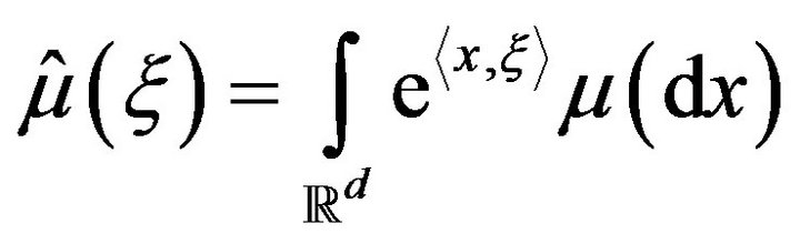
 where
where .
.
Then, the sequence of p.m.’s  satisfies the large deviations principle with constants
  and good rate function Ι:
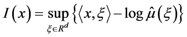
 where
where  is the dual space of Ε and

(in other words Theorem 2.1. is true).
Proof.
Let  be the family of finite-dimensional subspaces of
 , directed upward by inclusion. For each
 , let
, let  and
and
 the canonical projection of Ε onto
 , i.e.
 ; for each
 , let
, let  with
with
 be the canonical projection. The family
  is a projective system
( are finite-dimensional normed spaces)
and  satisfy the assumptions of Theorem 1.7, since:
i) The assumption implies that the sequence of p.m.’s.  is exponentially tight, since:

If t, a are constants, and r such that: 
 , we get
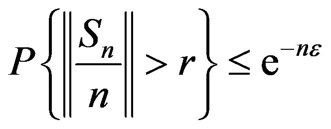 .
.
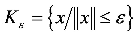
For given , we choose the (compact) set:
ii) For each  the sequence of p.m.’s
 satisfies the full large deviations principle with good rate function:
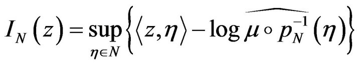 .
.
In fact, since:
 If we define the r.v.’s
 , they are i.i.d. with common distribution
  and values in the space
 . Also

from hypothesis, so using Cramer’s Theorem 2.1 (for finite dimensional spaces, see e.g. [1,4]), we have that the sequence of p.m.’s:

satisfies the large deviations principle with rate function
(using that ):
):

From i) and ii), and Theorem 1.7 we get that, the sequence of p.m.’s.  satisfies the large deviations principle with good rate function
 .
.
But: , so
, so

When someone deals with the empirical measures of an i.i.d sequence, the following large deviations result is true.
2) Theorem 2.3. (Sanov’s theorem in  for independent random variables)
Let  be a sequence of independent and identically distributed r.v.’s, taking values in
  with (common) distribution
 ,
,  the space of probability measures on
  equipped with the weak topology
 . Then:
1) a) (upper bound)  (weakly) closed:

with  Dirac’s measure defined on x, and
 (9)
(9)
(Kullback-Leibner information number or relative entropy of ν with respect to μ)
b) , the set
  is (weakly) compact.
2) (lower bound)  open:
open:

Remark 2.4. Theorem 2.3 is also true in the case of r.v.’s taking values in a complete separable topological space S and the space of probability measures P(S) is endowed with the weak topology (Donker-Varadhan (1976) and Bahadur-Zabell (1979) [1,5]). We prove now a generalization of Theorem 2.3 (the space P(S) is endowed with the τ-topology instead of the weak), using suitable projective systems. Also the r.v.’s are taking values on any set S which is endowed with a σ-algebra S (no need for topology on S).
Let  be a measurable space (i.e. S is any set and S a σ-algebra of subsets of S) and assume that the space
  is endowed with the τ-topology

where  the space of the bounded, S measurable maps
 ; convergence of nets of p.m.’s is defined in a similar way). Let also
 be the σ-algebra induced on
  by
by .
.
Theorem 2.5. (Sanov’s theorem for the τ-topology)
Let  be a sequence of i.i.d. r.v.’s, with (common) distribution
 , and values in the set S and S a σ-algebra of subsets of S. Then:
1) a) (upper bound) :
:

b) , the set
  is τ-compact.
2) (lower bound) :
:

Proof.
Let  and
and  the family of all finite subsets of
 , directed upward by inclusion. For
  is defined by:
  and for
 is the restriction map. It is easy to see that: Ι) the maps
  are
are  - measurable ΙΙ) the τ-topology on
 , is the initial topology induced by the maps
 , making the family
  a projective system.
If  and for
the probability measure:
 where
where  with
with 
defined by  and the r.v.’s
 are i.i.d
  -valued and
 .
.
Using 2.1. (for ), we get that the sequence of p.m.’s
  satisfies the large deviations principle with rate function:
i.e. condition i) of Theorem 1.7 is satisfied.
Also using an argument similar to that of Theorem 2.1 in [6], or else Lemma 2.1 [7] implies that , the set
 is τ-compact. This, using Lemma 2.2 [7], implies that

(condition ii) of Theorem 1.7). So, using Theorem 1.7, the sequence of p.m.’s  satisfies the large deviations principle with rate function
 .
.
3) Theorem (Sanov’s theorem for exchangeable r.v.’s)
Sanov’s Theorem 2.5 is still true in the case when the independence, as a dependence relation among the random variables of a stochastic process, is replaced by a weaker one described below.
Definition 2.6. Let  be r.v.s defined on the p.s.
  and values in the m.s.
 . We say that the r.v.’s are exchangeable or interchangeable [8], if the joint distribution of any κ of them
 , depends only on κ and not the specific r.v.’s. (the r.v.’s are identically distributed but not necessarily independent).
The notion of exchangeability is central in Bayesian Statistics and plays a role analogous to that played by i.i.d sequences in classical frequentist theory (in B.S. an exchangeable sequence is one such that future samples behave like earlier samples, meaning that any order of a finite number of samples is equally like). The bivariate normal distribution, the classical Polya’s urn model, any convex combination of i.i.d. r.v.’s, are some examples of exchangeable r.v.’s. An i.i.d sequence is (trivially) an exchangeable one and the same is true for a mixture distribution of i.i.d. sequences. A converse proposition (to this) is the well known, powerful result in the case of exchangeable sequences, de Finetti’s theorem.
Theorem 2.7. (de Finetti’s representation theorem)
If  is a sequence of exchangeable r.v.’s, then there is a probability space
  and transition probability function
 , i.e. a function such that:
a)  is a probability measure on S b)
  is a measurable function on Θ, and
 (10)
(10)
with  is the product measure on
  with all its components equal to
 . We say that, P is a mixture of the p.m.’s
  with mixing measure m.
Theorem 2.8. (Sanov’s theorem for exchangeable r.v.s in τ-topology)
Let  be a measurable space, the space
is endowed with the τ-topology and .
.
Let also  and:
and:
 (11)
(11)
Let  be a sequence of exchangeable r.v.’s taking values in S and suppose that the function
 is τ-continuous. Then:
1) If the space Θ is compact
α) (upper bound) :
:
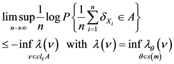
β) , the set
  is τ-compact.
2) (lower bound) :
:

Proof.
Using Theorems 2.1 and 2.2 [9], it is enough to prove:
whenever , the sequence of p.m.’s
  satisfies the large deviations principle with rate function
 .
.
We define the projective system  where
where
 the family of all finite subsets of
 , directed upward by inclusion,
  for
for , the map
  is defined by
and for  is the restriction map.
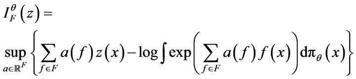
Finally . Then:
Ι) For : the p.m.

where 
 and the r.v.s
  are i.i.d (with respect to the p.m.
 ) with values in
 . The map:

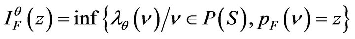
is jointly lower-semi-continuous, so using Theorem 3.1. [9] (or directly using Gartner-Ellis theorem), we get that the sequence of p.m  satisfies the large deviations principle with rate function:
II) It can be proved (in a way analogous to Theorem 2.1 Daras [6], see also the proof of Theorem 2.5) that
Finally, the result follows using Ι) and ΙΙ) and Theorem 1.7.
Remark 2.9.
a) Sanov’s theorem is true in a more general setting, namely when the p.m. P is a mixture of p.m.’s [6]. Then, Theorem 2.8 follows, as a corollary, using de Finetti’s theorem.
b) Theorem 2.8 extends a result of Dinwoodie and Zabell [9]. They prove their statement for a sequence
 of r.v.’s taking values in a Polish space S (no need here for topology on S) and the space
  is endowed with the weak topology (stronger than the τ-topology).
4) Moderate deviations
Let  be a positive real sequence such that:
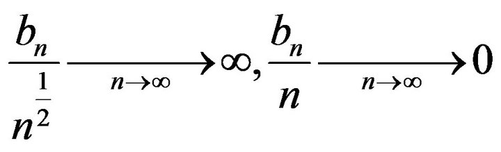 , (12)
and  a sequence of exchangeable r.v.s with distribution
  and for
 :
:
 (13)
(13)
Let  be the subspace of
  consisting of all those maps g, such that
 . Endow the space M(S) of finite signed measures on S with the topology
  generated by
 , i.e. the smallest topology making the maps of the form:
 continuous and let
 the σ-algebra induced on
  by
by . Then if
  and
and
 (14)
(14)
the following large deviations principle is true [6].
Theorem 2.10. (moderate deviations for empirical measures)
Let  be a sequence of exchangeable r.v.’s taking values in S. Assume that the map
 is τ-continuous. Then:
1) If the space Θ is compact, then a) (upper bound) :
:
 with
with
b) , the level set
  is τ- compact.
2) (lower bound) :
:
Remark 2.11.
a) Large deviations with normalizing constants of the form (12) are being called moderate deviations [6,10].
b) Theorem 2.10 generalizes Theorem 3.1. in [11].
There, the sequence  is based on a sequence of r.v.’s taking values in a m.s.
  and the space
  is endowed with the τ-topology.
c) Theorem 2.10 is true in general, namely when the p.m. P is a mixture of p.m.’s [6]. Then, Theorem 2.10 follows using de Finetti’s theorem.