1. Introduction
It would be difficult to exaggerate the influence of Newton’s theory of gravitation on the subsequent development of physics. As well as explaining Kepler’s laws of planetary motion, Newton’s theory was central to the successful mathematization of physics using the newly-invented calculus and it served as a paradigm for the later theories of electrostatics and magnetostatics. However, new insights into Milky Way satellite galaxies raise awkward questions for cosmologists: Do we have to modify Newton’s theory of gravitation as it fails to explain so many observations? In other words, although Newton’s theory does, in fact, describe the everyday effects of gravity on Earth, things we can see and measure, it is conceivable that we have completely failed to comprehend the actual physics underlying the Newton’s force of gravity. In addition, Newton’s theory does not fully explain the precession of the perihelion of the orbits of the Planets, especially of planet Mercury. Namely, it has been experimentally stated that the perihelion of Mercury’s orbits moves into the plane of its planetary motion around the Sun. In other words, all planetary motions of Sun’s planetary system depart from elliptical orbits obtained from Newton’s gravity theory, [1]. By the strict Schwarzshild-Droste’s solution to the static gravitational field with spherical symmetry, in the general Einstein’s relativity theory, the perihelion problem has been approximately solved, [1]. On the other hand, Einstein’s theory has some difficulties hard to be overcome such as the problem of singularity, that occurs in Newton’s theory too (all relevant physical variables, such as velocity, force, kinetic and potential energy, don’t exist at point of singularity). Accordingly, in order to solve simultaneously these two acutely vexed questions within Newton’s gravity theory, we present, in this research paper, an approximative modification of Newton’s gravity concept itself. The outline of this article is as follows: In the Preliminaries, the space-time continuum (the integral space), as an ambient space, is completely defined. In Section 1 we establish a causal connection between the expression for the kinetic energy of a material point and the Minkowski metric in the four-dimensional space-time continuum. In addition, in two separate subsections of this section we derive Newton’s equations of motion and the relativistic Hamilton-Jacobi equation for a free particle. Since the dynamic (Newton’s) equations of motion are formally derived from geodesic equations in Section 2, this section together with Appendix at the end of the paper provide a possibility of further work on the modification of Newton’s gravity theory in Section 3. In this last section we show that a comprehensive analysis of particle motion under the modified Newton’s gravity force leads to the perihelion motions of a Planet’s elliptical orbit.
2. Preliminaries
By a material point , introduced for the purpose of an useful idealization, one means a geometrical point, which is spatially no dimensional on the one hand and exactly fixed mass on the other. Closely related to the notion of a geometrical point is the set of values
  of some arbitrary
  variables
  denoting the contravariant co-ordinates of the real
  -dimensional configurative space. The geometrical point, defined by a set of zero values
 , is the zero co-ordinate point. If one of
  arbitrary variables
  is the time variable
 , then the space aforementioned becomes the space-time continuum (shortly called the integral space), [2]. As it was noted in [3] the value of
  is called moment or instant.
The set of all geometrical points of the spatial subspace of the integral space, to which the mass  can be joined in some strictly monotonous sequence of permitted instants of the time
 , makes an odograph usually referring to the a trajectory (motion path) of
 . The time variable
  is taken for a unique independent variable, so that all remaining spatial variables
  are functional variables. Across all the future text Greek indices take values
 , and Latin ones
 . In the space-time continuum the aforementioned trajectory of
  blossoms into an integral curve. The vectors
 and
and  defined with respect to the origin are position vectors of
  in the space-time continuum and in the spatial subspace of the integral space, respectively. The concept of a vector in vector hyper-dimensional spaces
  should be conditionally comprehended in the sense of its geometrical presentation in a form of segments. Hence it bears a name linear tensor, [4]. Covariant vectors
 , where
denotes , form a covariant vector basis
of the integral space. The vectors , such that at any point of the space
 , where the second order system
  (Kronecker’s delta-symbol, [5]) is the identity
  matrix, form a dual basis
  of
of
 . The differential
  of the position vector
of  is defined by
 , where the so called Einstein’s convention is applied to a summation with respect to the repetitive indexes (uppers and lowers), herein as well as in the further text of the paper.
3. The Action Metric in the Integral Space
Since the integral space is a metric affine space, whose linearly independent basis (fundamental) co-ordinate vectors reduced to the origin form an  -hedral basis, it follows that if
  is a line element of the metric affine space of the spatial continuum, then the expression for the kinetic energy
  of
of  can be stated in more appropriate form:
 (1)
(1)
considering the fact that the basic mechanical (kinematics and dynamics) parameters of  are its velocity
 , quantity of motion
 and kinetic energy
 . A term of
 , where
  is nominally equal to the light velocity in vacuum, can be added to both sides of the previous equation, as follows
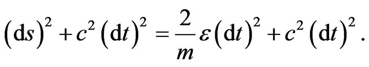 (2)
(2)
For  let
let  be such that
 . Then, (2) becomes
 (3)
(3)
This means that if , where
  is a line element of the metric affine space of the space-time continuum, then the four-dimensional integral space has the Minkowski metric, [1,4]. So, in this case the Minkowski metric (3) represents the kinetic energy
  of
of  in the integral space. Hence, the Minkowski metric
  is the kinetic metric of the integral space, [6].
If the Pfaff form  is absolute differential, that means that there exists a scalar valued function
  such that
 , then
  and
and
 (4)
(4)
where , and
, and  is the total mechanical energy of
 .
.
Now, we can start with the action  in the Lagrange sense along a motion path of
  in the integral space [4, 6],
 (5)
(5)
Since  it follows from (4) and (5) that
 (6)
(6)
Let us introduce an action line element , thoroughly explained in [6], in such a way that
 (7)
(7)
Accordingly, the action metric is as follows
 (8)
(8)
where

 are the metric tensors of
  and
and , respectively.
3.1. Newton’s Equations of Motion
By the well-known Maupertius-Lagrange’s principle [4], the path motion of  is just the path along which the action is stationary, more precisely along which the following two mutually equivalent conditions
 (9)
(9)
where  is the variational operator, are satisfied. By (7), the previous conditions are reduced to
 (10)
(10)
The second condition in (9) leads to the Euler Lagrange equations
 (11)
(11)
where  and
and

which yield Newton’s equations of motion
 (12)
(12)
3.2. The Relativistic Hamilton-Jacobi Equation for a Free Particle
Analyze (5) again, but now let  be a function of
 that means that
 . As
. As
 (13)
(13)
we introduce the functional , nominally equal to
 , such that
 (14)
(14)
as well as the functional  satisfying the condition
 (15)
(15)
which together with (15) yields
 (16)
(16)
since . Hence,
  is Lagrangian of
 . Further, since
  for
for , see (14), it follows from (15) that
  and
and
 (17)
(17)
The previous equation is the Hamilton-Jacobi one, so that  is the principal Hamilton’s functional of
 . Clearly, the Hamiltonian
  of
of  is equal to
 , more precisely to the integral of motion, considering the fact that the kinetic energy
  of
of  is a homogenous square function of
 . Now, by (14) and (15), we have
 , so that
 (18)
(18)
This together with (17) leads to the second form of the Hamilton-Jacobi equation
 (19)
(19)
In addition,
 (20)
(20)
which together with (8) yields
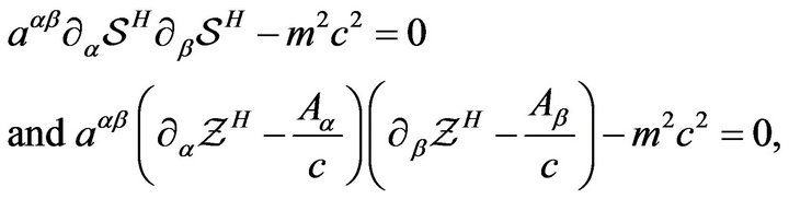 (21)
(21)
where . These two equations are obviously analogous to the relativistic Hamilton-Jacobi equation for a free particle, see [7,8].
4. The Binet Differential Equation
As is well-known from the tensorial analysis, see [6], all curves of the integral space, for which the condition (10) is satisfied, are geodesics, and the absolute Bianchi (covariant) derivative  of the unit tangent vector
 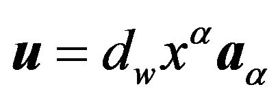 along geodesics is equal to zero (the vector projection of
  onto the tangent hyper-plane of the integral space is equal to zero). Thus, the geodesic equations are as follows
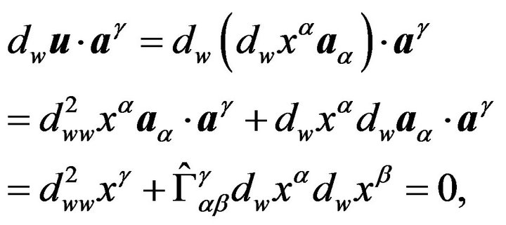 (22)
(22)
where  denotes
 , and
, and
 are the second kind Christoffel symbols with respect to the action metric space
 . Let
. Let . Since
 , see (8), it follows that
 (23)
(23)
where  are the second kind Christoffel symbols with respect to the Euclidean metric space
 . A new form of the geodesic equations (22), for a constrained material point
 , is as follows
 (24)
(24)
which yields
 (25)
(25)
since
 ,
,
 and
and .
.
So, (25) represents the Euler-Lagrange differential equations of the extremal curve in the explicit form, and at the same time Newton’s second law of motion under the action of a potential force  in the contravariant form:
 (26)
(26)
Accordingly, one may conclude that the dynamic (Newton’s) Equations (26) of motion are formally derived from the geometric Equations (22).
In the case of the free motion of , when
 , both the kinetic and action metric form of the integral space are pseudo-euclidean, while integral curves are straight-lines (see Appendix), as it was thoroughly explained in the monograph by [6]. On the other hand, the well-known Binet differential equation for central force motion of
 (27)
(27)
is obtained by differentiating (58) (see Appendix).
5. Modified Newton’s Gravity Concept
For the conservative Newton’s gravity force  the expression
  is as follows
 , where
  is the gravitational radius, so that (27) is reduced to
 (28)
(28)
where  and
and .
.
Since, in the limit as , Newton’s gravitational potential
  tends to infinity, it is logical to assume that
  is the first-order MacLaurin series approximation of the exponential function
 , so that
  and
and
 (29)
(29)
Accordingly, the modified Binet differential equation for the modified central Newton’s gravity force
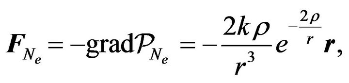 (30)
(30)
is as follows
 (31)
(31)
5.1. A motion Under the Action of 
Start with Newton’s second law of motion
 (32)
(32)
Multiply (32) on the right by the sector velocity vector  as follows
 (33)
(33)
Since  it follows from (33) that
 (34)
(34)
where the vector  satisfying the relation
  is no longer an element of Milankovic’s constant vector elements, more precisely is no longer Laplace’s integration vector constant, see [9]. If we now multiply
  by
by , we get
 (35)
(35)
Since , it follows from (35) that
 (36)
(36)
where  is an angle between
  and
and . This equation describes the motion of
  under the action of the modified Newton’s gravity force
 . Conditionally speaking, there is no formal difference between (36) and its analog in the ordinary Newton’s gravity theory. The key difference lies in the fact that
  is no longer constant vector.
For  let
let  and
and , where
  is the unit vector orthogonal to
 . Then, from (34) we get
 (37)
(37)
which together with (36) yields
 (38)
(38)
where  and
and
 .
.
In addition, the dot product  leads to
 (39)
(39)
Thus,
 (40)
(40)
If  is the angle between
  and
and , it follows from (36) and (40) that
 (41)
(41)
Hence,
 (42)
(42)
Note that , whenever
 . If we now multiply (38) by
  we get
 (43)
(43)
which together with (41) and (42) yields
 (44)
(44)
whenever . If
. If , then
 (45)
(45)
Since , see (38), it follows from (36) that
 (46)
(46)
which together with (45) finally yields
 (47)
(47)
This result we can also get explicitly from (46). Namely, if  is the polar angle, then
 . Therefore, it follows from (46) that
 (48)
(48)
Since  we have
 (49)
(49)
that is just the same as (47). Hence,
 (50)
(50)
So, as , where
  and
and  are the semimajor axis and the eccentricity of the orbit, the following angle value
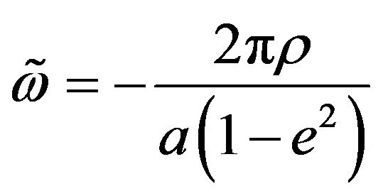 (51)
(51)
is a very good approximation for the perihelion regression  per one revolution
  of the Planets.
5.2. The Modified Perturbing Force
If, in addition to the modified Newton’s gravity force , we include the modified perturbing force [10]

where  and
and  are the radial vector between the Planet and the perturbing planet (whose orbit is assumed to be circular and coplanar with Mercury’s orbit) and the gravitational radius for the perturbing planet, respectively, then

where  is the angle between
  and
and , and
, and  is the unit vector perpendicular to
 . Thus, the second equation of (35) becomes

where  and
and

This vector is the modified Laplace’s integration vector (or more precisely, the modified Laplace-RungeLenz vector). Their original versions come from the ordinary Newton’s gravity theory. If we denote

by , then we have

6. Conclusion
The mathematical model of a material point motion in the three-dimensional spatial subspace of the four-dimensional space-time continuum and in the field of the action of a conservative active force  is analogous to Newton’s mathematical model of the classical mechanics. In addition, the metric
  of the integral space, which represents the kinetic energy of a material point from the viewpoint of that space, is the Minkowski metric from Einstein’s relativity theory. Accordingly, it can be said that in the paper a new connection has been established, in contrast to an approximative one, between the classical Newton’s mathematical model and the relativistic Einstein’s mathematical model.
On the other hand the approximately modified Newton’s gravity concept is not, from any point of view, in collision with old Newton’s one. At the same time it solves the acutely vexed questions within old Newton’s gravity concept (the singularity and perihelion problems). Furthermore, analyzing the analytical expression for the modified Newton’s gravity force , we can separate the four indicative domains of its field of the action (see Figure 1). The first one is a domain of the weak action on finitely small distances. The second one is a domain
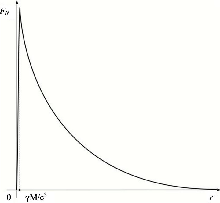
Figure 1. Modified Newton’s gravity force.
of the strong action in a neighborhood of the gravitational radius
 . The third one is a domain of the action on finitely large distances relative to the gravitational radius
  and with the relatively small velocities relative to the light velocity, and the fourth on finitely large distances relative to the gravitational radius
  and with velocities that are comparable to the light velocity. Previously separated domains of the field of the action of the modified Newton’s gravity force
  it would be desirable to compare to the fields of the action of the four so far non-unified fundamental forces (weak and strong nuclear interactions, gravity and Lorenz’s electromagnetism). Clearly, all of these facts aforementioned could be subject of further analyses. Note at the end that a correction to Newton’s gravity law in the form of the functional dependence
 irresistibly reminding of the modified Newton’s gravity force, and obviously wrongly called the fifth force, has been revealed by a reexamination of the old attraction data and careful new force measurements presented in [11].
Appendix: The Freee Motion of  in the Integral Space
Let us start with the Euler-Lagrange equations
 (52)
(52)
where
 (53)
(53)
as the condition for the action (12) to be stationary. The geodesic Equations (13) are explicitly obtained from it in a known way. If spatial co-ordinates are spherical ones , then the components of
  depend only on
  and
and , so that it follows from (52) that
 (54)
(54)
and
 (55)
(55)
that leads to
 (56)
(56)
and
 (57)
(57)
Let the polar extension  and the polar angle
  be intensities of
  and an angle between the position vector
  and the polar axis
  passing through the origin and the perihelial point, respectively. Then, since
 , where
  is the so-called sector velocity vector, it follows from the condition (57) that the motion is the plane one
  and
and . As
. As  then we obtain finally from (5), (10) and (57) that
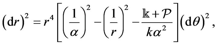 (58)
(58)
that just leads to the Binet differential equation for free motion in plane polar co-ordinates
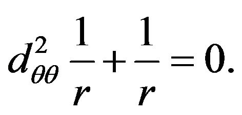 (59)
(59)
The solution , where
 is the perihelial distance, to this differential equation, defines a straightline in plane polar co-ordinates.