1. Introduction
The complex physical phenomena are depicted of nonlinear evolution equations (NLEEs) which are widely used as models. One of the fundamental problems is to establish their traveling wave solutions. As a result, the attention of searching traveling wave solutions of NLEEs is enhancing and has now become a hot topic to researchers. At present time, various methods have been established to obtain exact solutions. For example, the Hirota’s bilinear transformation method [1,2], the Backlund transformation method [3,4], the truncated Painleve expansion method [5,6], the inverse scattering method [7], the weierstrass elliptic function method [8], the homogeneous balance method [9], the Jacobi elliptic function expansion method [10-13], the generalized Riccati equation method [14], the tanh-coth method [15-19], the F-expansion method [20,21], the direct algebraic method [22], the Cole-Hopf transformation method [23], the Exp-function method [24-30] and others [31-36].
Recently, Wang et al. [37] presented a widely used method to construct traveling wave solutions of different nonlinear partial differential equations (PDEs), called the basic  -expansion method. In addition, in this method
  is executed as traveling wave solutions, where
  Later on, many researchers established exact traveling wave solutions of various nonlinear PDEs via this method. For example, Feng et al. [38] studied the well-known Kolmogorov-Petrovskii - Piskunov equation to obtain analytical solutions by using the same method. Naher et al. [39] constructed abundant traveling wave solutions of the higher-order CaudreyDodd-Gibon equation via this powerful method. In [40], Abazari and Abazari concerned about the same method for obtaining hyperbolic, trigonometric and rational function solutions of Hirota-Ramani equation. Zayed [41] investigated some nonlinear evolution equations in mathematical physics to establish exact solutions by applying this method. Jabbari et al. [42] obtained some solutions of the coupled Higgs equation and the Miccari system via the same method while Ozis and Aslan [43] implemented the
  -expansion method to construct traveling wave solutions of the Kawahara type equations using symbolic computation. In [44], Gepreel studied some nonlinear PDEs with variable coefficients in mathematical physics by applying the same method for constructing exact solutions. Elagan et al. [45] executed this method to obtain innovative solutions of the generalized FitzHugh-Nagumo equation. Borhanifar and Moghanlu [46] established some solutions for the Zhiber-Sabat equation and other related equations via the same method whilst Borhanifar and Abazari [47] investigated two generalized form of Burgers equation for constructing general solutions by using the
  -expansion method. In [48], Wang et al. constructed explicit solutions of the generalized (2+1)-dimensional Zakharov-Kuznetsov equation via this method and so on.
Many researchers studied the fourth order Boussinesq equation to construct analytical solutions by using different methods. For instance, Zhang [49] implemented the F-expansion method to investigate this equation for obtaining traveling wave solutions. In [50], Wazwaz employed the extended tanh method to construct exact solutions of the same equation.
The importance of this work is, the fourth order Boussinesq equation is considered to construct new exact traveling wave solutions including solitons, periodic and rational solutions by applying the basic  -expansion method.
2. The Basic  -Expansion Method
Suppose the general nonlinear partial differential equation:
 (1)
(1)
where  is an unknown function,
  is a polynomial in
  and the subscripts stand for the partial derivatives.
The main steps of the basic  -expansion method [37] are as follows:
Step 1. Consider the traveling wave transformation:
 (2)
(2)
where  is the wave speed. Now using Equation (2), Equation (1) is converted into an ordinary differential equation for
 (3)
(3)
where the superscripts indicate the ordinary derivatives with respect to 
Step 2. According to possibility, Equation (3) can be integrated term by term one or more times, yields constant(s) of integration. The integral constant may be zero, for simplicity.
Step 3. Suppose that the traveling wave solution of Equation (3) can be expressed in the form [37]:
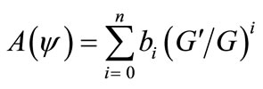 (4)
(4)
with  satisfies the second order linear ODE:
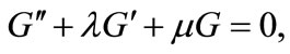 (5)
(5)
where  and
and  are constants.
Step 4. To determine the integer n, substituting Equation (4) along with Equation (5) into Equation (3) and then taking the homogeneous balance between the highest order nonlinear terms and the highest order derivatives appearing in Equation (3).
Step 5. Substituting Equations (4) and (5) into Equation (3) with the value of  obtained in Step 4. Equating the coefficients of
  then setting each coefficient to zero, we obtain a set of algebraic equations for
  and
and 
Step 6. Solve the system of algebraic equations which are obtained in Step 5 with the aid of algebraic software Maple and we obtain values for  and
and  Then, substitute obtained values in Equation (4) along with Equation (5) with the value of n, we can obtain the traveling wave solutions of Equation (1).
3. Applications of the Method
In this section, the fourth order Boussinesq equation involving parameters is investigated to establish traveling wave solutions including three different families by applying the  -expansion method.
3.1. The Fourth Order Boussinesq Equation
In this work, we consider the fourth order Boussinesq equation followed by Wazwaz [50]:
 (6)
(6)
Boussinesq established Equation (6) to illustrate the propagation of long waves in shallow water. This equation also arises in other physical applications, for example, iron sound waves in plasma, nonlinear lattice waves and in vibrations in nonlinear string. Further, the details of this equation can be found in references [49-54].
Equation (6) is integrable, therefore, integrating with respect  twice and setting the constants of integration equal to zero, yields:
 (7)
(7)
Taking the homogeneous balance between  and
and  in Equation (7), we obtain
Therefore, the solution of Equation (7) is of the form:
 (8)
(8)
where  and
and  are constants to be determined.
Substituting Equation (8) together with Equation (5) into the Equation (7), the left-hand side of Equation (7) is converted into a polynomial of  According to Step 5, collecting all terms with the same power of
 . After that, setting each coefficient of the resulted polynomial to zero, yields a set of algebraic equations (for simplicity, which are not presented) for
  and
and 
Solving the system of obtained algebraic equations with the help of algebraic software Maple, we obtain two different values.
Case 1.
 (9)
(9)
where  and
and  are free parameters.
Case 2.
 (10)
(10)
where  and
and  are free parameters.
Substituting the general solution Equation (5) into Equation (8), we obtain three different families of traveling wave solutions of Equation (7):
Family 3.1.1. Hyperbolic function solutions:
when  we obtain
 (11)
(11)
If U and V are taken as specific values, various known solutions can be rediscovered.
Family 3.1.2. Trigonometric function solutions:
when  we obtain
 (12)
(12)
If U and V are taken as specific values, various known solutions can be rediscovered.
Family 3.1.3. Rational function solution:
when  we obtain
 (13)
(13)
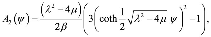
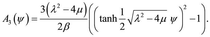
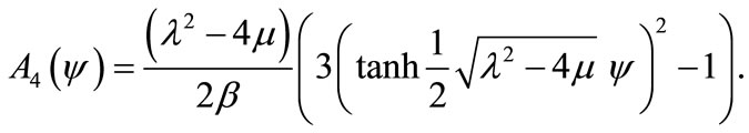
Family 3.1.1.1. Hyperbolic function solutions:
Substituting Equations (9) and (10) together with the general solution Equation (5) into the Equation (8), yields the hyperbolic function solution Equation (11), our traveling wave solutions become respectively (if  but
but ):
):
where

where

Again, substituting Equations (9) and (10) together with the general solution Equation (5) into the Equation (8), yields the hyperbolic function solution Equation (11), we obtain following exact solutions respectively (if  but
but ):
):
Moreover, substituting Equations (9) and (10) together with the general solution Equation (5) into the Equation (8), we obtain the hyperbolic function solution Equation (11), our obtained wave solutions become respectively (if ):
):
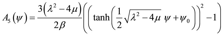
where 

where 
Family 3.1.2.1. Trigonometric function solutions:
Substituting Equations (9) and (10) together with the general solution Equation (5) into the Equation (8), yields the trigonometric function solution Equation (12), we obtain following solutions respectively (if  but
but ):
):

where 

where 
Also, substituting Equations (9) and (10) together with the general solution Equation (5) into the Equation (8), yields the trigonometric function solution Equation (12), our solutions become respectively (if  but
but  ):
):
Furthermore, substituting Equations (9) and (10) together with the general solution Equation (5) into the Equation (8), yields the trigonometric function solution Equation (12), our obtained traveling wave solutions become respectively (if ):
):

where 
where 
Family 3.1.3.1. Rational function solutions:
Substituting Equations (9) and (10) together with the general solution Equation (5) into the Equation (8), we obtain the rational function solution Equation (13), and our wave solutions become respectively (if  = 0):
= 0):
where 
where 
4. Results and Discussion
It is worth declaring that some of our obtained solutions are in good agreement with already published results which are presented in Table 1. Moreover, some of obtained exact solutions are described in Figures 1-12.
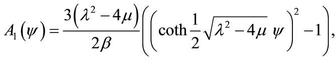
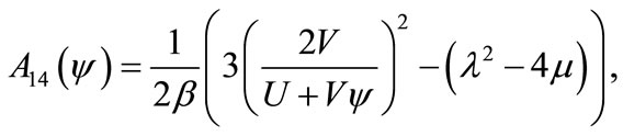
Beyond this table, we obtain new exact traveling wave solutions A1, A3, A5, A6, A7, A9, A11, A12, A13, and A14,
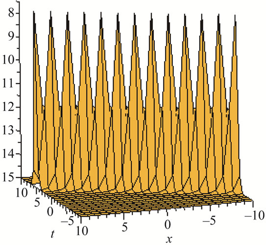
Figure 1. Solutions solution for λ = 3, μ = 1, α = 3, β = 1.

Figure 2. Periodic solution for λ = 6, μ = 8, α = 12, β = 9.
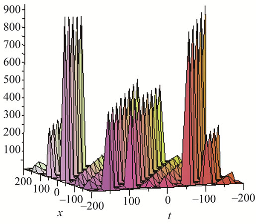
Figure 3. Solitons solution for λ = 3, μ = 3, α = 9, β = 5.
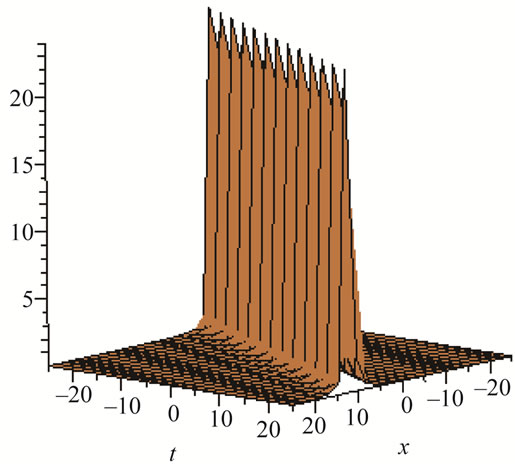
Figure 4. Solitons solution for λ = 4, μ = 4, α = 0.5, β = 1, U = 0.5, V = 1.

Figure 5. Solitons solution for λ = 3, μ = 2, α = 7, β = 2.
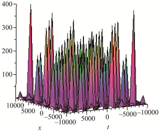
Figure 6. Solitons solution for λ = 4, μ = 5, α = 11, β = 9.
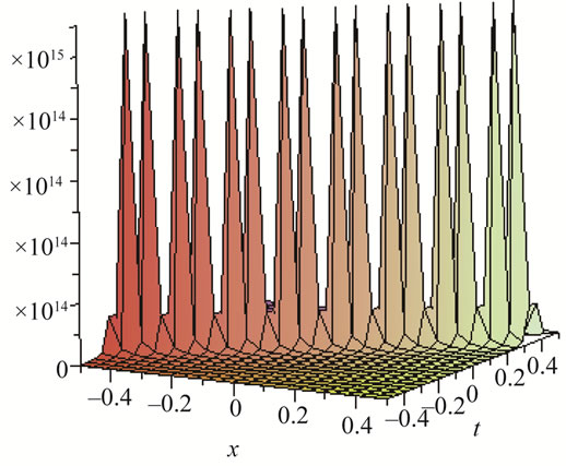
Figure 7. Solitons solution for λ = 4, μ = 4, α = 1.5, β = 5 × 10–11, U = 0.75, V = 24.

Figure 8. Periodic solution for λ = 3, μ = 3, α = 16, β = 15.
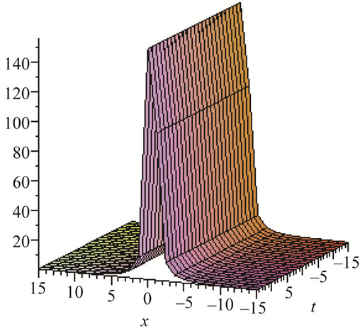
Figure 9. Periodic solution for λ = 8, μ = 16, α = 5 × 10⁻⁶, β = 0.125, U = 5, V = 9.
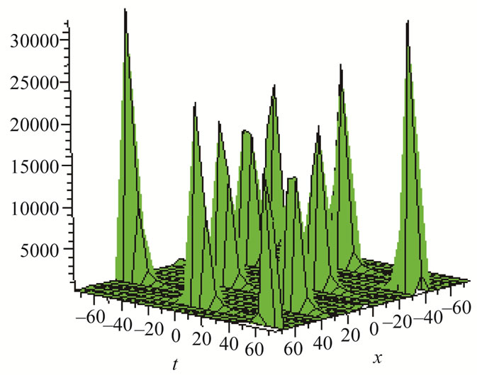
Figure 10. Solitons solution for λ = 5, μ = 7, α = 15, β = 0.5.
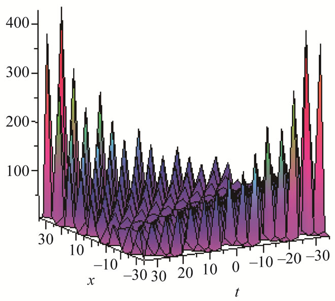
Figure 11. Solitons solution for λ = 5, μ = 7, α = 7, β = 1.
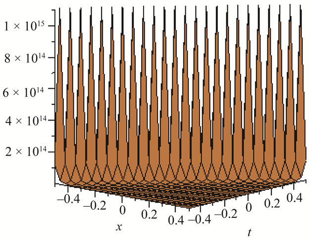
Figure 12. Solitons solution for λ = 6, μ = 9, α = 1, β = 5 × 10–11, U = 0.75, V = 24.
which are not being established in the previous literature.
5. Conclusion
In this article, the basic  -expansion method with second order linear ordinary differential equation is implemented to investigate the fourth order Boussinesq equation involving parameters. The obtained solutions are presented through the hyperbolic functions, the trigonometric functions and the rational functions. Further, it is important mentioning that some of our solutions are coincided with published results and others have not been stated in earlier literature. The solutions show that this method is reliable and straightforward solution method to obtain exact solutions of nonlinear evolution equations. Therefore, this powerful method can be effectively used to construct new exact traveling wave solutions of diffe

Table 1. Comparison between Wazwaz [50] solutions and newly obtained solutions.
rent nonlinear partial differential equations.
6. Acknowledgements
The authors would like to express their thanks to the referee(s) for their valuable comments and suggestions.