A Cubic Spline Method for Solving a Unilateral Obstacle Problem ()
1. Introduction
Let  be a bounded open domain in
  with smooth boundary
 , and let
  be an element of
  with
with  on
on . Set
. Set

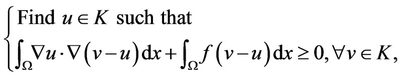
We consider the following variational inequality problem:
 (1)
(1)
where f is an element of . This problem is called a unilateral obstacle problem. It is well known that problem (1) admits a unique solution u, and if
 , then u is an element of
  (see [1,2]). There are several alternative solution methods of the obstacle problem; see, e.g., [1,3-5]. Numerical solution by penalty methods have been considered, e.g. by [4,6]. In this paper we develop a numerical method for solving a one dimentional obstacle problem by using the cubic spline collocation method and the generalized Newton method. First, problem (1) is approximated by a sequence of nonlinear equation problems by using the penalty method given in [2,7]. Then we apply the spline collocation method to approximate the solution of a boundary value problem of second order. The discret problem is formulated as to find the cubic spline coefficients of a nonsmooth system
 , where
 . In order to solve the nonsmooth equation we apply the generalized Newton method (see [8-10], for instance). We prove that the cubic spline collocation method converges quadratically provided that a property coupling the penalty parameter
  and the discretization parameter h is satisfied.
Numerical methods to approximate the solution of boundary value problems have been considered by several authors. We only mention the papers [11,12] and references therein, which use the spline collocation method for solving the boundary value problems.
The present paper is organized as follows. In Section 2, we present the penalty method to approximate the obstacle problem by a sequence of second order boundary value problems. In Section 3 we construct a cubic spline to approximate the solution of the boundary problem. Section 4 is devoted to the presentation of the generalized Newton method. In Section 5 we show the convergence of the cubic spline to the solution of the boundary problem and provide an error estimate. Finally, some numerical results are given in Section 6 to validate our methodology.
2. Penalty Problem
Let  be an element of
  with
with  on
on . Assume that
  is an element of
 , then the solution u of problem (1) is an element of
  and can be characterized as (see [1], for instance):
 (2)
(2)
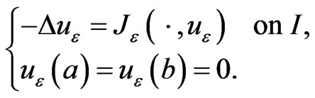
The penalty problem is given by the following boundary value problem (see [10], p. 107, [12]):
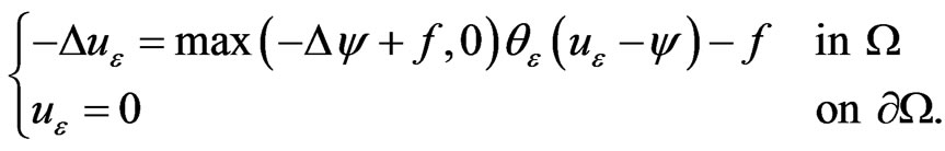 (3)
(3)
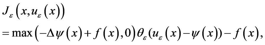
where  is a sequence of Lipschitz functions which tend to the function
  defined by
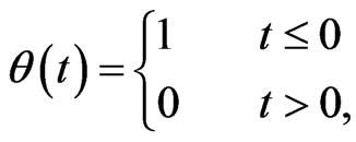 (4)
(4)
almost everywhere on , as
, as  goes to zero. Assume that the function
 ,
,  , is uniformly Lipschitz, non increasing and satisfy
 . Then problem (3) admits a unique solution (see [2] p. 107). We now specify the function
 (5)
(5)
We have the interesting properties.
Theorem 1 ([2,7]) Let u denote the solution of the variational inequality problem (1) and ,
,  , denotes the solution of the penalty problem (3) with
  defined by relation (5). Then
  is a nondecreasing sequence and

3. Cubic Spline Collocation Method
In this section we construct a cubic spline which approximates the solution  of problem (3), with
  is the interval
  and
and  is the function given by (5).
Cubic Spline Solution
Let
be a subdivision of the interval I. Without loss of generality, we put , where
  and
and .
.
Denote by  the space of piecewise polynomials of degree 3 over the subdivision
  and of class
  everywhere on
 . Let
. Let ,
,  , be the B-splines of degree 3 associated with
 . These Bsplines are positives and form a basis of the space
 . If we put
 (6)
(6)
then problem (3) becomes
 (7)
(7)
It is easy to see that  is a nonlinear continuous function on
 ; and for any two functions
  and
and ,
,  satisfies the following Lipschitz condition:
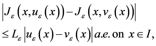 (8)
(8)
where

Now, we define the following interpolation cubic spline of the solution  of the nonlinear second order boundary value problem (7).
Proposition 2 Let  be the solution of problem (7). Then, there exists a unique cubic spline interpolant
 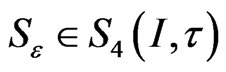 of
of  which satisfies:
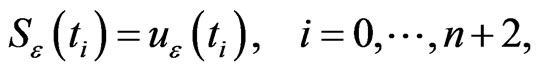
where ,
,  ,
,  ,
,  and
and .
.
Proof Using the Schoenberg-Whitney theorem (see [13]), it is easy to see that there exits a unique cubic spline which interpolates  at the points
 ,
,  .
.
If we put , then by using the boundary conditions of problem (7) we obtain
 , and
, and
Hence 
Furthermore, since the interpolation with splines of degree d gives uniform norm errors of order  for the interpolant, and of order
  for the
  derivative of the interpolant (see [13], for instance), then for any
  we have
 (9)
(9)
The cubic spline collocation method, that we present in this paper, constructs numerically a cubic spline 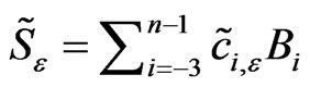 which satisfies the Equation (7) at the points
 ,
, . It is easy to see that
and the coefficients ,
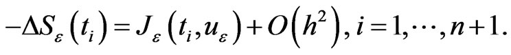
,  , satisfy the following nonlinear system with n + 1 equations:
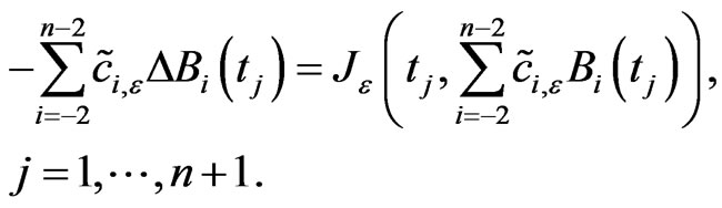 (10)
(10)
Relations (9) and (10) can be written in the matrix form, respectively, as follows
 (11)
(11)
where
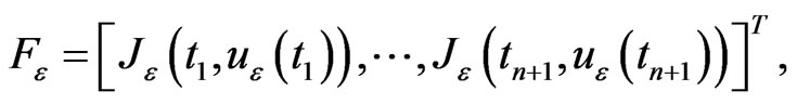

and  is a vector where each component is of order
 . It is well known that
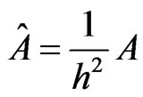 , where A is a matrix independent of h given as follows:

Then, relation (11) becomes
 (12)
(12)
with  is a vector where each one of its components is of order
 .
.
The results of this work are basically based on the invertibility of the matrix A. Then, in order to prove that A is invertible we give the flowing lemma.
Lemma 3 (de Boor [13]) Let  such that
  on
on  where
where . If S admits r zeros in
  then
then .
.
Proposition 4 The matrix A is invertible.
Proof Let  be a vector of
such that . If we put
 , then we have
  and
and  for any
 . Since
  then
then . If we assume that
  in
in , then using the above lemma and the fact that
  has
has  zeros in
 , we conclude that
 , which is impossible. Therefore
  for each
 . This means that the function S is a piecewise linear polynomial in I. Since
 , then we obtain
  for any
 . Consequently
  and the matrix A is invertible.
Proposition 5 Assume that the penalty parameter  and the discretization parameter h satisfy the following relation:
 (13)
(13)
Then there exists a unique cubic spline which approximates the exact solution  of problem (7).
Proof From relation (12), we have . Let
. Let  be a function defined by
 (14)
(14)
To prove the existence of cubic spline collocation it suffices to prove that  admits a unique fixed point. Indeed, let
  and
and  be two vectors of
 . Then we have
 (15)
(15)
Using relation (8) and the fact that , we get
where . Then we obtain
From relation (15), we conclude that
Then we have
With 
by relation (13). Hence the function  admits a unique fixed point.
In order to calculate the coefficients of the cubic spline collocation given by the nonsmooth system
 (16)
(16)
we propose the generalized Newton method defined by
 (17)
(17)
where  is the unit matrix of order
  and
and  is the generalized Jacobian of the function
 , (see [8-10], for instance).
4. Generalized Newton Method
Let  be a function. Consider the equation

The Newton method assumes that F is Fréchet differentiable, and is defined by
 (18)
(18)
where  is the inverse of the Jacobian of the function F. However, in nonsmooth case
  may not exists. The generalized Jacobian of the function F may play the role of
  in the relation (18). Rademacher's theorem states that a locally Lipschitz function is almost everywhere differentiable (see [14], for instance). Assume that F is a locally Lipschitz function and let
  be the set where F is differentiable. We denote
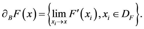
The generalized Jacobian of F at ,
,  , in the sense of Clarke [15] is the convex hull of
 :
:
 (19)
(19)
For nonsmooth equations with a locally Lipschitz function F, the generalized Newton method is defined by
 (20)
(20)
where  is an element of
 . If the function F is semismooth and BD-regular at x, then the sequence
  in (20) superlinearly converges to a solution x (see [8,9, 16,17]). A Function F is said to be BD-regular at a point x if all the elements of
  are nonsingular, and it is said to be semismooth at x if it is locally Lipshitz at x and the limit

exists for any . The class of semismooth functions includes, obviously smooth functions, convex functions, the piecewise-smooth functions, and others (see [10,18], for instance). Since the function
  defined by (6) is a Lipshitz and piecewise smooth function on
 , then the function
  given by (14) is also a Lipshitz and piecewise smooth function on
 . Hence we may apply the generalized Newton method to solve the problem (16).
5. Convergence of the Method
Theorem 6 If we assume that the penalty parameter  and the discretization parameter h satisfy the following relation
 (21)
(21)
then the cubic spline  converges to the solution
 .
.
Moreover the error estimate  is of order
 .
.
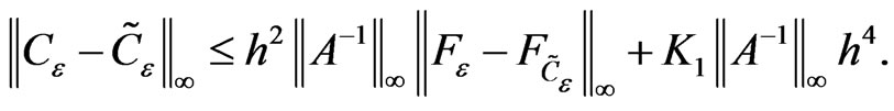
Proof From (12) and Lemma 4, we have
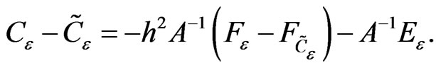
Since  is of order
 , then there exists a constant
  such that
 . Hence we have
 (22)
(22)
On the other hand we have
Since  is the cubic spline interpolation of
 , then there exists a constant
  such that
 (23)
(23)
Using the fact that
 (24)
(24)
then, we obtain
By using relation (22) and assumption (21) it is easy to see that
 (25)
(25)
We have
Then from relations (23), (24) and (25), we deduce that  is of order
 . Hence the proof is complete.
Remark 7 Theorem 6 provides a relation coupling the penalty parameter  and the discretization parameter h, which guarantees the quadratic convergence of the cubic spline collocation
  to the solution
  of the penalty problem.
6. Numerical Examples
In this section we give numerical experiments in order to validate the theoretical results presented in this paper. We report numerical results for solving a one dimensional obstacle problem by using the cubic spline method to approximate the solution of the penalty problem (7), and the generalized Newton method (20) to determine the coefficients of the cubic spline collocation. Consider the obstacle problem (1) with the following data: ,
,  and
and
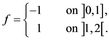
The true solution  of this problem is given by

As a stopping criteria for the generalized Newton’s iterations, we have considered that the absolute value of the difference between the input coefficients and the output coefficients is less than .
.
Tables 1-4 show, for different values of the discretization parameter h, the error between the cubic spline collocation  and the true solution u. We note the convergence of the solution
  to the function u depends on the discretization parameter h and the penalty parameter
 . Theorem 6 implies that for a fixed h, this convergence is guaranteed only if there exists
  such that
 . Some experimental values of
  are given in Tables 1-4.
Theorems 1 and 6 imply that we have the error estimate between the exact solution and the discret penalty solution is given by . The obtained results show the convergence of the discret penalty solution to the solution of the original obstacle problem as
the parameters h and  get smaller provided they satisfy the relation (21). Moreover, the numerical error estimates behave like
  which confirms what we were expecting.
7. Concluding Remarks
In this paper, we have consider an approximation of a unilateral obstacle problem by a sequence of penalty problems, which are nonsmooth equation problems, presented in [2,7]. Then we have developed a numerical method for solving each nonsmooth equation, based on a cubic collocation spline method and the generalized Newton method. We have shown the convergence of the method provided that the penalty and discret parameters satisfy the relation (21). Moreover we have provided an error estimate of order  with respect to the norm
 . The obtained numerical results show the convergence of the approximate penalty solutions to the exact one and confirm the error estimates provided in this paper.
NOTES