Energy Portfolio Management with Entry Decisions over an Infinite Horizon ()
1. Introduction
Climate change is now recognized as the major environmental problem facing the world. The factor of most concern that causes climate change is the increase in carbon dioxide levels due to emissions from fossil fuel combustion. Therefore, construction of an alternative power plant is crucial to reducing carbon dioxide emission. By introducing an alternative plant, the firm therefore has an energy portfolio. A decision on when a new plant should be built must consider this uncertainty due to fluctuations in electricity prices. We study this problem with the optimal entry decision for the new plant, given fixed capital investment and the optimal dispatch decision for the conventional plant and the alternative plant with the objective of maximizing the long-term expected profit under geometric Brownian motion for the electricity prices over an infinite horizon.
Investments in and operations of power plants have been widely studied. Deng et al. [1] valued electricity derivatives by futures-based replication due to the nonstorable nature of electricity. Tseng and Barz [2] evaluated a power plant in the short-term with unit commitment constraints using a real-options approach. By the same approach, Tseng and Lin [3] evaluated a power plant involving processes of electricity and fuel prices. Thompson et al. [4] studied the valuation and optimal operations of hydroelectric and thermal power generators through an optimal control and partial-integral-differential-equations (PIDEs) approach. Takashima et al. [5] analyzed the optimal entry strategy of two firms under price uncertainty and competition with real options and game theory. Recently, Deng et al. [6] studied the same problem over a finite time horizon, and solved the resulting partial differential equation (PDE) by finite difference method. Liu [7] studied the optimal time to abandon a plant of a firm with a portfolio of two plants over an infinite horizon by stochastic control approach, and the optimal policy is obtained in closed-form.
This paper studies the timing that a firm invests in a new technology. We assume the firm owns a plant, and considers adding a new plant while maximizing the expected long-term profit. Since the firm can generate electricity by a portfolio of two plants, the optimal dispatch of these two plants needs to be determined after the new plant is constructed. (Admittedly, it is possible to include more plants with various generating methods; we discuss this extension in Section 5. Under the geometric Brownian motion of long-term electricity prices [8], we formulate the decision problem as a mixed stochastic control problem. Due to the intractability of the mixed problem, we decompose it into two auxiliary problems: one is a regular stochastic control problem, the other one is an optimal stopping problem. The solution to the auxiliary problems is equivalent to the original control problem, and is obtained in closed-form.
Our contribution is two-fold: First, we formulate the problem as a mixed stochastic control problem. Therefore, the optimal entry decision and optimal dispatch are addressed accordingly. To the best of our knowledge, the mixed control problem cannot be solved directly. Second, we decompose the intractable mixed problem into two auxiliary problems, and the corresponding value functions satisfy a standard Hamilton-Jacobi-Bellman (HJB) equation or variational inequality (VI). We obtain the closed-form solutions to the value functions.
The rest of the paper is organized as follows. We formulate the decision problem as a non-standard stochastic control problem in Section 2. In Section 3, we write the equivalent form of the value function to the control problem. By standard arguments, we obtain the closedform of the value function. In Section 4, we provide a numerical example to confirm our results and sensitivity analysis. Finally, conclusions and future research directions are presented in Section 5.
2. Problem Formulation
We introduce the following notation to formulate the problem.
•  : Electricity price [$/MWh]
•  : the risk-adjusted discount rate
•  : maximum proportion of total wealth invested in alternative method (AL)
•  : proportion of total wealth invested in AL [Decision variable]
•  : Production rate of the conventional method (CON)
•  : Production rate of AL
•  : Total cost of generating
  units of electricity from CON
•  : Total cost of generating
  units of electricity from AL
•  : time to construct AL [Decision variable]
•  : capital investment for constructing AL [\$]
We assume the long-term electricity price follows the standard geometric Brownian motion [8]:
 (1)
(1)
where μ and σ are expected growth rate and volatility of the electricity price respectively, and {Bt} is a Wiener processes. Assume x is the initial position of electricity price. That is, X0 = x.
The objective of the firm is to choose an optimal stopping time τ to construct AL, and an optimal proportion α after τ in order to maximize the expected profit. If we define the expected discounted profit functional J given initial electricity price x, proportional investment in AL α, and the time to construct AL τ as
 (2)
(2)
subject to (1), where Ex is the expectation with respect to x and αt is obviously a function of time t, then the value function u is defined as
 (3)
(3)
where Γ is the set of stopping times.
3. Solution Methods
In order to solve the non-standard stochastic control problem (3), we proceed as follows: By introducing an auxiliary function x, we obtain the equivalent function w to the value function u, which solves an optimal stopping problem. We then get the closed-form solution of w by value-matching and smooth-pasting conditions.
3.1. Equivalent Problem to (3)
We define the auxiliary function v as the expected profit from the portfolio assuming AL is constructed:
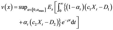 (4)
(4)
It is easy to get
 (5)
(5)
by the fact that , where
 (6)
(6)
If we define the value function w as
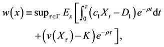 (7)
(7)
we can formally prove that w is equivalent to u in (3) (See [9]).
The value function w satisfies the combination of variational inequality of optimal stopping problem as follows
 (8)
(8)
where the generator L is defined as
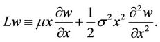 (9)
(9)
3.2. Closed-Form Solution to w
First we consider the solution to the following ordinary differential equation (ODE):
 (10)
(10)
A special solution  to (10) can be easily identified as
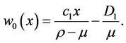 (11)
(11)
If we try a function w of the form
 , for some constant β, (12)
we get
 (13)
(13)
where
 (14)
(14)
Note that
 (15)
(15)
Therefore if we assume , then we can get there exists
  such that
Next we solve for the explicit form of solution to Problem (7). With the value of , we put
 (16)
(16)
for constants C and  to be determined.
By value matching condition [10] at , we have
 (17)
(17)
and smooth pasting condition [10] at , we have
 (18)
(18)
It is easy to see that
 (19)
(19)
and
 (20)
(20)
(20) requires that
 (21)
(21)
Therefore we obtain
 (22)
(22)
(20) also requires that
 (23)
(23)
Plugging (22) into (20) yields
 (24)
(24)
In summary, the value function u is equivalent to w, which has the closed-form (16). The unknown constants are determined by (22) and (24) with constraints (23).
4. Numerical Example and Sensitivity Analysis
A numerical example with the following parameters

The results are as follows

They indicate that when electricity price is higher than 91.97, it is optimal to construct the alternative plant. Otherwise, the decision-maker needs to keep the conventional method.
Next we carry about sensitivity analysis by changing one of the given parameters to see how it affects the threshold level  as in (22).
First we change the capital investment K from $400 to $600 with other parameters fixed. Figure 1 shows the threshold level  increases linearly from $81.76 to $102.2 as K increases. This confirms the result of (22) and is consistent with the intuition that higher capital investment discourages the firm from constructing the new plant.
Second, if the electricity price growth rate μ changes from 1% to 3% with other parameters fixed, then the threshold level  decreases from $84.38 to $77.47 as shown in Figure 2. This result explains the fact: the higher the electricity price, the earlier a firm tends to construct the new plant. Figure 2 also shows a nonlinear relationship between the growth rate μ and the threshold level
  as in (14) and (22).
Third, if the electricity price volatility σ changes from 10% to 200% with other parameters fixed, then the threshold level  increases drastically from $84.38 to $2372.1 as shown in Figure 3. This impact of price volatility can be explained analytically from (14) and (22): as volatility σ is the leading term of quadratic Equation (14), it has huge impact on the solution β and the threshold level
  through (22).

Figure 1. Sensitivity analysis with capital investment K.

Figure 2. Sensitivity analysis with electricity price growth rate μ.
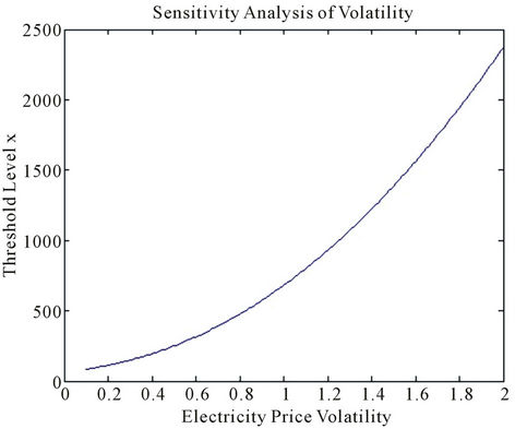
Figure 3. Sensitivity analysis with electricity price volatility σ.
We omit the sensitivity analysis with other parameters as it is straightforward to carry out given (22).
5. Conclusions
We study the optimal entry decision for alternative plant given a fixed capital investment, and the optimal dispatch decision between the conventional plant and the alternative plant. By introducing two auxiliary problems, we solved the mixed stochastic control problem in closed form.
This paper can be generalized in the following ways. First, the analysis in this paper is just based on one stochastic process (the electricity price); we admit that there are other stochastic processes that can affect the decisions, such as the cost of the carbon dioxide emission. We would have more stochastic processes in addition to electricity prices process, and we need to solve the multidimensional optimal control problem. Second, switching costs will be incurred when we abandon the conventional method, and singular control technique would be employed to study this problem.