Complex Valued Recurrent Neural Network: From Architecture to Training ()
1. Introduction
Current paper aims to give the complete guidance from the state space models with complex parameters to the complex valued recurrent neural network of a special type. This paper is unique in translating the models suggested by Zimmermann in [1] to the complex valued case. Moreover one can see unique approach for managing the problems with transition functions which arise in complex-valued case, new approach for treating the error function which gives the unique advantages for the complex-valued neural networks. A lot of research in the area of complex valued recurrent neural networks is currently ongoing. One can find the works of Mandic [2,3], Adali [4] and Dongpo [5]. Mandic and Adali pointed out the advantages of using the complex valued neural networks in many papers. This paper will supply the neural network community with new architecture which shows better results in its complex-valued case.
We start the paper with the description on the state space models and then proceed with the very detailed explanations regarding the complex valued neural networks. We discuss complex valued system identification, error function properties in its complex valued case, complex valued back-propagation and break points with transition functions. Paper ends up with the small discussion on applications and advantages which arise form the complex valued case of the considered architecture.
State space techniques may be used to model recurrent dynamical systems. There are two principle ways of modeling dynamical systems: 1) use a feed-forward neural network and use delayed inputs or 2) use a recurrent architecture and model the dynamics itself. The first approach is based on Takens theorem [6] that a dynamical system or the attractor of the dynamical system can be reconstructed by a set of previous values of the realizations of the dynamical system (expectations). This is true for chaotic systems, but in real world applications feed forward networks cannot be used for forecasting the states of dynamical systems. Therefore, recurrent architectures are the only sensible way of forecasting dynamical systems, i.e. to represent the dynamics in the recurrent connection weights. This approach was first suggested by Elman [7] and later extended by Zimmermann [8]. As an example for this paper we will consider the so called open-system for which we will build a state space model based on the recurrent complex valued neural network. Such an open-system (open means that the system is driven not only by its internal state changes but also by external stimuli) is given as follows:
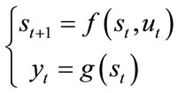 (1)
(1)
Here, the states of the system ( ) depend on the previous states as well as some system input
  through some non-linear function f. The output of the system depends on the current state of the system mapped through another non-linear function g. A graphical representation is in Figure 1.
In the rest of this paper, we will use networks described by Equation (1) and Figure 1. In order to generalize the approach, we now assume that the dynamic system’s behavior is described by complex numbers, which means that  and functions
 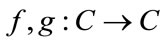 are defined on the domain of complex numbers.
2. Complex Valued Neural Network
The Complex Valued Recurrent Neural Network (further CVRNN) is a straight forward generalization of the realvalued RNN. The algorithms which are used for CVRNNs can be also used for RNNs without loss of generality. To describe the CVRNN we start with a feed-forward path, and then we will discuss the error back-propagation algorithm (further CVEBP) and the training of such architectures.
2.1. Architecture Description and Feed Forward Path
The system represented by Figure 1 and Equation (1) can be realized as follows (as suggested by Zimmermann [9]): consider a set of 3-layer-feed-forward networks (further FFNN), whose hidden layers are connected to each other. This connection represents the evolution of the corresponding dynamical system inside the RNN. The structure of this type of network is shown in Figure 2.
The dynamical system develops based on 1) internal evolution of the system state governed by the matrix A and the activation function. Matrices B, C convert the external stimulus to the state (in the sense of data compression) and produce the output from the state (state decompression). Therefore, one can write the following system of equations, which describe the system in Figure 2.

Figure 1. Dynamical system representation.
 (2)
(2)
where we have selected  as an activation function
 , which performs the non-linear transformation of the state. Thus, all temporal relations of the dynamical system are represented in the matrix
  (to be learned during training), the compression, and the decompression ability represented by the matrixes B, C respectively (note that all elements of matrixes
 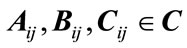 are complex numbers).
One word about the weights matrices: the matrices between the layers are always the same (suggested as the “shared weights concept” in [8]). It is exactly this property that makes this network recurrent. Next, we will discuss the back propagation for the shared weights concept.
Summarizing, the RNN has actuation inputs ; it has observable outputs
 , it has states
 , which evolve under the regime of the matrix
 , and it has a non-linear activation function
 .
.
2.2. Error Back Propagation for the CVRNN
The first variant of Complex Valued Error Back Propagation was described by Haykin in [7]. First, we have to define the error function. Since, in the complex valued case there are no “greater/less than” relations, the output of the error function must be a real number in order to make it possible to evaluate the training result and to guide it into the direction of an error reduction. The procedure of the whole network training is as follows: find the network parameters, which are those weights that produce the minimum of the error function:
 (3)
(3)
where w are weights, f is the activation function, u are the complex valued inputs of the system, and  are observables.
One class of functions, which produces real-valued output from complex arguments, is the following:
 (4)
(4)
where the over bar denotes complex value conjugate .
.
This current error function is not analytic, i.e., the derivative  is not defined over the entire range of input values. Therefore, back propagation cannot be applied.
The requirement for the analyticity of any function E is given by the Cauchy-Riemann conditions:
 (5)
(5)
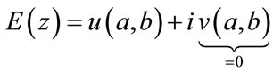
where the function E is described with the following equation:
 (6)
(6)
where 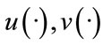 are some real differentiable functions of two real variables.
The requirement for the error function to produce real output means that .
.
 (7)
(7)
If we want , we have to take an error function similar to (4) since our error function
 , the optimality conditions are given by:
 (8)
(8)
The function  makes a mapping of the following type:
  instead of
 . In order to calculate the derivative of the function
  one should use the so called Wirtinger derivative (discussed, e.g., in Brandwood [10]): the Wirtinger derivative with respect to z and
  can be calculated in the following way:
 (9)
(9)
For the real functions of complex variables 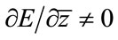 therefore the minimization of the error function can be done in both directions
  or
or .
.
Now we have the derivatives of the error function defined in the Wirtinger sense.
Note that this error function “minimizes” the complex number, which in the Euler notation (see Equation (10)) would mean, that it minimizes both amplitude and phase of the complex number, which is in our case  :
:
 (10)
(10)
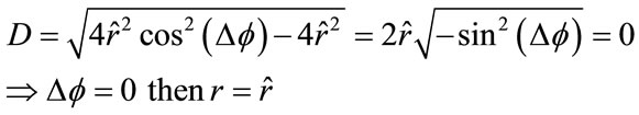
This error function has very unique and desirable properties. Let us describe these properties more in detail. We rewrite (4) into Euler notation:
 (11)
(11)
The discriminant of (11) is negative and only can be equal to zero that the equation has 1 root:
We can also rewrite (4) in the following way:
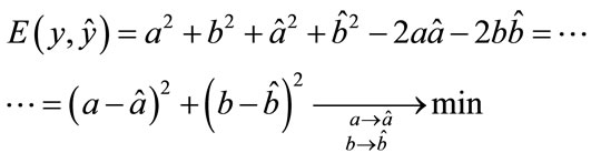 (12)
(12)
One can see that error function (4) minimizes both real and imaginary parts of the complex number.
After defining a suitable error-function, we can now start with the CVEBP description. The procedure for CVEBP is shown in Figure 3. It follows the description in [9] or the RNN. The “ladder” algorithm allows a local and efficient computation of the recurrent network partial derivatives of the error with respect to the weights. The advantage of the algorithm shown in Figure 3 is that it intelligently unites the equations, the architecture and the locality of the CVEBP.
In Figure 3, one can see the CVEBP which is done for the shared matrix  and for the case when all NN parameters are complex numbers.
2.3. Weights Update Rule for the CVRNN
In order to find the training rule for the weights update, we introduce the Taylor expansion of the error function:
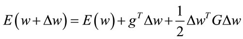 (13)
(13)
where (one can note that  has to be equal to the

Figure 3. Complex valued error back propagation for the derivatives with respect to .
.
that Taylor expansion exist):
 (14)
(14)
Following Johnson in his paper [11], two useful theorems to calculate the derivatives can be applied.
Theorem 1. If the function  is real-valued and analytic with respect to
  or
or , all stationary points can be found by setting the derivatives in Equation (9) with respect to either
  or
or  to zero.
Theorem 2. By treating  and
and  as independent variables, the quantity pointing in the direction of the maximum rate of change of
  is
is 
The proof of the theorems was demonstrated by Johnson in [11].
Following Karla in [12] and Adali in [13], if minimization goes in the direction of , then
  . Otherwise, if we minimize in the direction of
 , it results in
  which need not necessarily be negative. This will lead us in the direction of a different minimization.
Following Theorem 2 and Equation (7), we consider
 . The Taylor expansion exists, since the derivatives are defined and we can obtain a training rule for the optimization of weights in the direction of
 :
:
 (15)
(15)
Notice that Figure 3 is very similar to the real valued RNN, despite the conjugations instead of the transposes.
One should also note that this error function is universal because it optimizes both the real and the imaginary part of the complex number. It has a simple derivative, and it is a parabola, which means it has only one minimum and smooth bounds. A typical convergence of the error during the training is presented in Figure 4.
Note that this error function is a real value. Figure 4 shows the modulus, i.e., exactly the error function, the angle error is:
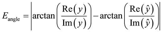 (16)
(16)
After presenting the CVEBP and discussing the convergence of the error, we now discuss the final aspect of the CVRNN, which is the activation (or transition) function.
2.4. Activation Function in the Complex Valued Domain
It is well known that for real valued networks, one of the requirements for the activation function is to be continuous (ideally: bounded), and it should have at least one derivative defined for the whole search space.
Unfortunately, this is not the case for the complex valued functions due to the Liouville theorem [10]. Moreover, all transition functions which are not linear have an unlimited growth at their bounds (example: sine-function) or have singularity points an (example is the tanh-function, see Figure 5 below).
Based on the following Theorem 3, we can make several remedies:
Liouville Theorem 3. If a complex analytic function is bounded and complex differentiable on the whole complex plain, it is constant.
This theorem has been proven in Remmert [14].
Remedy 1. Choose bounded functions which are only real valued but not complex differentiable:
 (17)
(17)
Remedy 2. Constrain the optimization procedure in order to stay in the area, where there are no singularities:

Figure 4. Error convergence for the absolute part of the error (dashed line) and for the phase of the error (solid line).

Figure 5. Absolute part behavior of the tanh function: it shows two singularities, which are periodic at π/2.
 (18)
(18)
Remedy 3. All real analytic functions are differentiable in complex domain using the Wirtinger Calculus.
One can also try to substitute the problematic regions of the functions with different functions which do not have the problem in the following region (the problem is the presence of singularity point) following the (19) below:
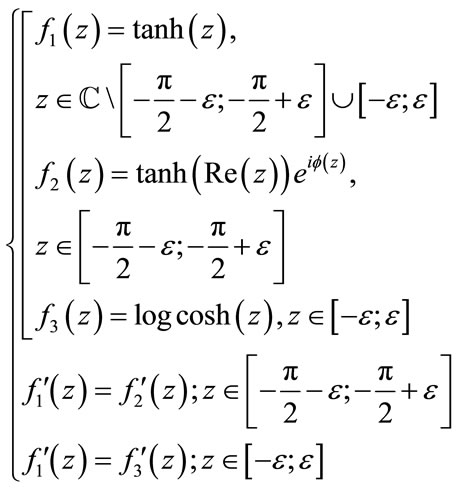 (19)
(19)
The result of such experiment is shown in Figure 6 below.
Typical use of the CVRNN with the activation function  will be possible with the non-linear function, as long as the weights are initialized with small numbers and the error minimization goes in the correct direction (i.e., the error decreases and steps of the weight update becomes smaller as training time increases). Also, the weights do not go above 1, which means they do not approach the singularities of the function.
3. Summary and Outlook
In this paper we discussed several aspects of CVRNN.

Figure 6. The transition function for the substitute functions.
We showed the architecture of the CVRNN, discussed the feed forward operation as well as the back-propagation CVEBP and the weights update rules. We discussed problems with the activation and error functions and showed how to overcome these problems.
There are many advantages of using CVRNN: continuous time modeling, modeling of electrical devices and energy grids, robust time series prediction, physical models of the brain, etc. Future work will focus on applications and evaluation of CVRNNs.