Switch to Devalued Drachma and Cost-Push Inflation: A Simple Input-Output Approach to the Greek Case ()
1. Introduction
At the end of 2009, the Greek economy experienced serious internal and external imbalances. Large “twin deficits” on the budget and current accounts (12% and 10% of GDP, respectively, in 2010), high public debt and net international investment position ratios (145% (103%) and –98% (–44%) of GDP, respectively, in 2010 (2000)), negative net national savings (17% of net national disposable income in 2010, and, with the exception of the year 2001, they were negative in each year of the period 2000-2010), high ratios of gross (net) profits to wages (130% (100%) in 2010, and the average value of the period 2000-2010 is 149% (118%)) and unemployment (12% in 2010 and 18% in August 2011) are the current problems of the economy. The exit of Greece from the Eurozone, and the reintroduction of drachma, is viewed by some scholars as the catastrophe of the economy and by others as its salvation. It may be argued, however, that the “number one” problem is the lack of international competitiveness, whilst all the other problems constitute epiphenomena ([1,2]). So, the “late-2000s financial crisis” was not the “cause” but rather the occasion of the “Greek crisis”.
Within the Economic Monetary Union (EMU), the division of labour tends to be governed by the “law of absolute (and not comparative) advantages”, since there is 1) deactivation of trade (tariff and non-tariff) policies; 2) a single currency; 3) free movement of money capital; 4) free movement of labour force; and 5) the so-called “Stability and Growth Pact” ([3-5] and [6-8]). Consequently, the national economies (and/or the regions of certain national economies), which are characterized by a low productivity, will eventually not be able to produce any commodity (setting aside the non-tradable commodities) or, in the best-case scenario, will produce only certain commodities (i.e. “unskilled labour-intensive” commodities; see also [9]). All the available empirical data suggest that this tends to be the case for the Greek economy (e.g. [10]). Therefore, under the present circumstances, i.e. within the EMU, the contemplation of internal devaluation policies, such as reduction in government expenditures and cuts in unit labour costs in the private sector, seems to be the only available, although too little too late “remedy” (see also [11]).
This paper uses simple dynamic input-output price models and data from the most recent (2005) Symmetric Input-Output Table (SIOT) of the Greek economy to estimate the effects of an external devaluation on the cost-push inflation rate.1 All the models have the same structure, which is imposed by the available SIOT (it provides no data on fixed capital stocks, non-competitive imports and sectoral employment), but they are based on different assumptions about the response of sectoral gross value added to currency devaluation. These models have been formed and applied in [13], and the findings were consistent with empirical evidence on the rate of imported cost-inflation in the first year after the last drachma devaluation (by 14%) in March 1998 (the estimated values were in the range of 1.16% - 1.75% and the “actual” one was almost 1.2%).2 The remainder of the paper is structured as follows. Section 2 outlines the analytic framework. Section 3 presents the data construction. Section 4 presents the empirical results. Section 5 concludes.
2. The Analytic Framework
Consider an open, linear system involving only single products and basic commodities (in the sense of Sraffa [15]; see also [16]). Furthermore, assume that 1) the production period is uniform across all industries; 2) the input-output coefficients are fixed; 3) there are no noncompetitive imports; 4) at least one commodity enters directly into its own production; and 5) the system is viable, i.e. the Perron-Frobenius (P-F hereafter) eigenvalue of the irreducible and primitive  matrix of total input-output coefficients,
  , is less than 1.3 On the basis of these assumptions we can write
 (1)
(1)
or
 (1a)
(1a)
where 
 denotes the stationary price vector of domestically produced commodities,
  ,
,  the irreducible and primitive matrices of domestic and imported input-output coefficients, respectively,
  ,
,  the nominal exchange rate,
  the given vector of foreign currency prices of the imported commodities,
  , and
, and 
 the vector of gross values added per unit activity level, which equals the sum of 1) consumption of fixed capital,
 ; 2) net taxes on production,
 ; 3) net operating surplus,
 ; and 4) compensation of employees,
  , or
, or
 (2)
(2)
(e.g. [17]). By solving Equations (1) and (1a) for  we obtain
 (3)
(3)
where  and
and  denotes the identity matrix.
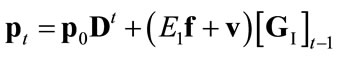
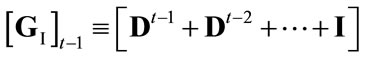
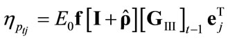
In order to analyze the effects of nominal exchange rate changes on prices we use the following well-known dynamic version of system (1a) ([18-21]):
 (4)
(4)
where ,
,  denotes the rate of devaluation, and
  (see Equation (3)). Now we shall distinguish between the following three cases (for a critique of this treatment, see [22]):
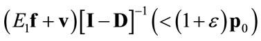
1) . Then the solution of Equation (4) is
 (4.I)
(4.I)
where
 ,
,
 denotes the elasticity of
  with respect to the nominal exchange rate,
  , and
, and  tends to
as  tends to infinity, since
  and, therefore,
 .
.
2) , where
 . Then the solution of Equation (4) is
 (4.II)
where
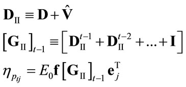
and  tends to
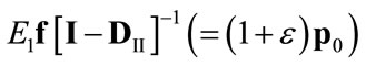 since
since  (
( implies that the P-F eigenvalue of
  equals 1 and, therefore,
  ).
).
3) , where

(see Equation (2)),  ,
,  (see Equation (2)) and
 . Then the solution of Equation (4) is
 (4.III)
where
 ,
,
 ,
,
 and
and  tends to
 since
since .
.
Thus, it can be concluded that, within these models, the price movement is governed by the “dated quantities”
([15]) of imported inputs, i.e. ,
,  ,
,  and
and , which reflect the technical and social conditions of production.
3. Data Construction
The SIOT of the Greek economy are provided via the Eurostat website (http://ec.europa. eu/eurostat), and describe 59 product/industry groups, which are classified according to CPA (Classification of Product by Activity). However, all the elements associated with the industry “Uranium and thorium ores” equal zero, whilst the only positive elements associated with the industry “Private households with employed persons” are “compensation of employees” and “final consumption expenditure by households” (which are equal to each other). Therefore, we remove these industries from the analysis and derive SIOT of dimensions 57 × 57.
The market prices of all products are taken to be equal to 1; that is to say, the physical unit of measurement of each product is that unit which is worth of a monetary unit (e.g. [23]). Thus, the matrices of input-output coefficients and the vector of gross values added per unit activity level (as well as its constituent components; see equation (2)) are obtained by dividing element-by-element the inputs and the gross value added of each industry, respectively, by its gross output.
Finally, we set , and given that the international competitiveness of the Greek economy has declined by almost 30% since 2001 (in accordance with estimates of the Bank of Greece; e.g. [10]), we suppose that
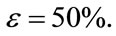
4. Empirical Results
The application of the three models (see Equations (4.I)- (4.III)) to the input-output data of the Greek economy, for the year 2005, gives the results summarized in Tables 1-3 (Mathematica 7.0 is used in the calculations, whilst the precision in internal calculations is set to 16 digits. For the analytical results, which are available on request from the authors, see [24]).
Tables 1 and 2 are associated with Model III, which gives the highest rates of cost-inflation. Table 1 reports the industries that exhibit the three largest and the three smallest price increases after the devaluation, the relevant price evolution, and some statistical measures (i.e. the arithmetic mean, AM, standard deviation, SD, and coefficient of variation, CV  SD (AM)–1) for the entire price vector. Table 2 reports the evolution of the AM of commodity prices of the four major sectors of the economy (ν indicates the number of industries and the numbers in parentheses indicate the SD), and the percentage of sectoral exports (imports) to total exports (imports). Thus, since the price movement is governed by the dated quantities of imported inputs, it can be concluded, roughly speaking, that 1) Manufacturing (“Agriculture” and Services) is (are) the most (less) import-dependent sector(s); 2) Manufacturing (“Agriculture”) is the most (less) dependent sector on direct imported inputs (as judged by
 , which equals the change in the P-F price eigenvector); and 3) the production conditions are similar across all industries in the “Mining” sector (as judged by the SD of commodity prices).
As is well known, the adjustment of Model III (for example) towards the new equilibrium depends on the magnitudes of  (which are in the range of 1.248 - 18.862) and
  (
( 0.893; see also Fig-
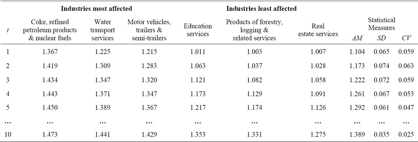
Table 1. The post-devaluation largest and smallest price increases; Model III.

Table 2. The price evolution of the four major sectors; Model III.
ure 1, which displays the location of the “relative eigenvalues”,  and
and ,
,
 in the complex plane). Indeed, the simulations show that the speed of the inflationary “wave” is not too high: the ΑΜ of commodity prices associated with Model III (II) reaches approximately 95% of its final (asymptotic) value at
 , with
  0.023 (
 ), whilst that of the less realistic Model I remains practically unchanged, and approximately equal to 1.093, with
  0.065, for
 .4
.4
Table 3 is associated with the three models and reports the evolution of the per-period cost-inflation rate (as measured by the gross value of domestic production), . It then follows that at
  the international competitiveness of the economy (as measured by the real exchange rate,
 ) increases by