Efficient Pricing of European-Style Options under Heston’s Stochastic Volatility Model ()
1. Introduction
Stochastic volatility models such as the model of Heston (1993) [1] are a frequent choice among finance researchers and practitioners to approximate stock price dynamics. Popularity of Heston’s model stems from its ability to reproduce a number of important time-series features of stock prices that are not adequately captured by geometric Brownian motion dynamics. In particular, Heston’s model is able to account for the leverage effect, that is, an increase in the volatility of a stock when its price declines, and a decrease in the volatility when the price rises (for more details, see Aït-Sahalia and Kimmel, 2007 [2]). As such, the model is often employed when pricing derivative securities, since it helps to correct for empirical deficiencies of the famous Black and Scholes’ (1973) [3] formula (for a discussion, see Aït-Sahalia and Lo, 1998 [4]).
Under Heston’s dynamics, the values of Europeanstyle options cannot be expressed in closed form. Instead, they may be computed numerically using the transform methods of Duffie et al. (2000) [5] and Bakshi and Madan (2000) [6], which require inverting the characteristic function of an underlying state price vector. The characteristic function can be expressed analytically using Heston’s original solution, or alternatively obtained as a special case of a more general solution of Zhylyevskyy (2010) [7]. This paper applies a particularly suitable inversion procedure and exploits symmetry properties of characteristic functions, in order to derive a computationally efficient formula for the value of a European-style put. The value of a European-style call is obtained using a parity relationship for European-style derivatives. Exploiting the symmetry of the characteristic function allows for a reduction of the domain of integration in the inversion, and cuts roughly in half the time needed for option valuation.
Efficient pricing of European-style options under Heston’s dynamics is important from a practical standpoint, since many single-name and index equity options listed on organized exchanges are European-style. Also, values of the European-style options may be used in methods of calculating prices of derivative securities of a different style, for example, in the Geske-Johnson method (Geske and Johnson, 1984 [8]) of pricing American-style options using a compound-option technique (for an implementation, see Zhylyevskyy, 2010 [7]).1
2. Stock Price Dynamics
The financial market is assumed to admit no arbitrage opportunities. Thus, there is a risk-neutral probability measure, denoted here as P, under which discounted asset prices are martingales (Harrison and Kreps, 1979 [13]). One of the traded assets is a riskless bond fund with a share worth  at time t, where
  is some initial value and
  is a risk-free rate. It will be convenient to use this bond fund as a numéraire security and discount asset prices by
  when appropriate.
The dynamics of a stock price,  under P are described by a system of stochastic differential equations
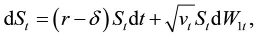 (1)
(1)
 (2)
(2)
where  stands for a dividend rate,
  represents an unobservable squared volatility,
  and
and  are correlated standard Brownian motions on a filtered probability space
  with
with  and
and , and α, β, and γ are nonnegative constants satisfying a restriction
  in order for
  to be almost surely positive (Chernov and Ghysels, 2000 [14]).
To derive values of European-style options, it will be convenient to work with a log-price,  Applying Ito’s lemma to Equation (1), the evolution of the logprice is described by a stochastic differential equation
 (3)
(3)
3. Characteristic Function
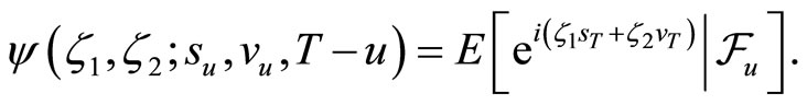
Let τ denote the time duration between current date t and some future date T,  Given the log-price
  and squared volatility
  the conditional characteristic function of the state vector
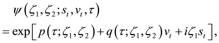
  is
is
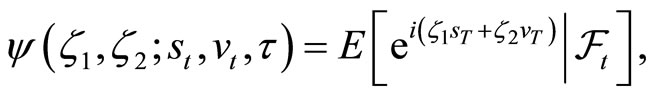
where E is the expected value taken under P and  and
and  are real-valued arguments.
Likewise, the conditional characteristic function of  at a date
  is
is
Since , the σ-field
 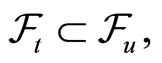 and therefore,
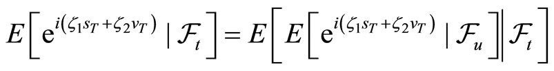 by the law of iterated expectations. Thus,
 (4)
(4)
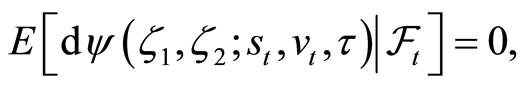
by taking u arbitrarily close to t. Applying Ito’s lemma to ψ it follows that
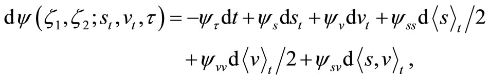
where  and
and  denote
  and
and , respectively. Then, Equations (2), (3), and (4) imply that ψ solves a partial differential equation
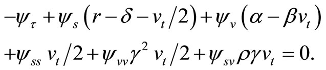 (5)
(5)
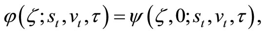
Zhylyevskyy (2010) [7] provides a complete solution for ψ using Equation (5). For reference, the solution is outlined in the appendix. The marginal conditional characteristic function of the log-price , which will be inverted to derive the value of a European-style put, is obtained as a special case:
 (6)
(6)
where  is a real-valued argument.
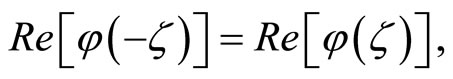
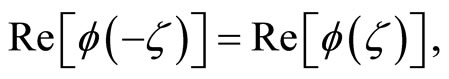
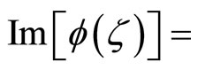
The complex-valued function  is symmetric in the sense that its real part is an even function,
while its imaginary part is an odd function,
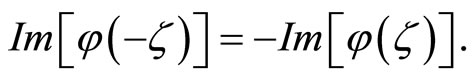
This symmetry will allow for a simplification of the option value’s expression and is a property of all characteristic functions, as Lemma 1 shows.
Lemma 1. Let  be the characteristic function of a random vector Y, where
  is a real-valued vector of the same dimension as Y. The real part of
  is an even function,
and the imaginary part of  is an odd function,


 .
.
Proof. By definition, 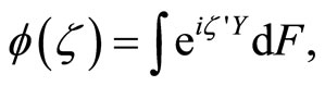 where F is the cumulative distribution function of Y. Applying Euler’s formula,
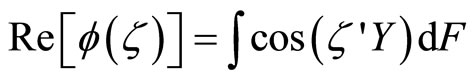
and 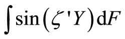
 .
.
It then follows from the properties of trigonometric functions that
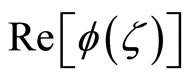
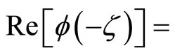
and 
 .
.
4. Option Value Formulas
This section applies the transform methods of Duffie et al. (2000) [5] and Bakshi and Madan (2000) [6], and exploits the symmetry of the characteristic function φ to obtain computationally efficient formulas for values of European-style puts and calls under Heston’s dynamics. Initial steps of the derivation follow the approach of Epps (2004) [15], but the idea to exploit the symmetry of the characteristic function is novel.
Let  denote the current value of a European-style put with a strike price X, given the (current) underlying stock’s price
  volatility
  and time to expiration
  The put is allowed to be exercised on date T when its value will be
  =
=  The first fundamental theorem of asset pricing implies that the put’s value, discounted by the share price of the riskless bond fund, is a martingale. Thus,

and therefore,
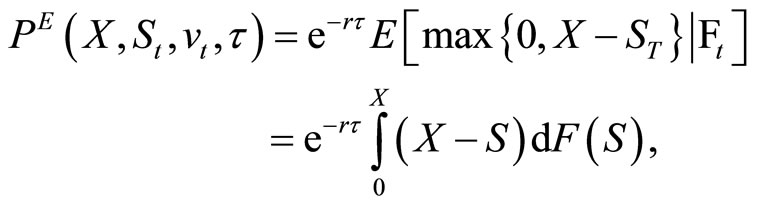
where F is the conditional cumulative distribution function of . Note that
  since the stock price cannot be negative. Integrating
  by parts, the put’s value can be expressed as
Observe that

where G is the conditional cumulative distribution function of the log-price  Hence, by changing variables as
  the put’s value can be re-expressed as
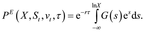 (7)
(7)
The characteristic function φ can be inverted to obtain G as follows (Gil-Pelaez, 1951 [16]):
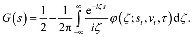 (8)
(8)
Plugging Equation (8) into Equation (7),
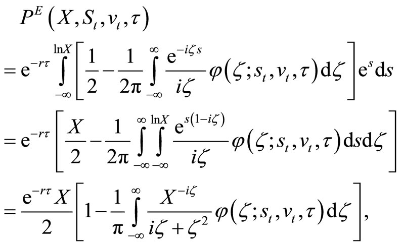 (9)
(9)
where the change in the integration order after the second equality sign is due to Fubini’s theorem.2
The put option value formula, Equation (9), can be simplified by exploiting the symmetry of φ. Denoting the complex-valued integrand in Equation (9) as 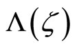 and applying Euler’s formula to it,
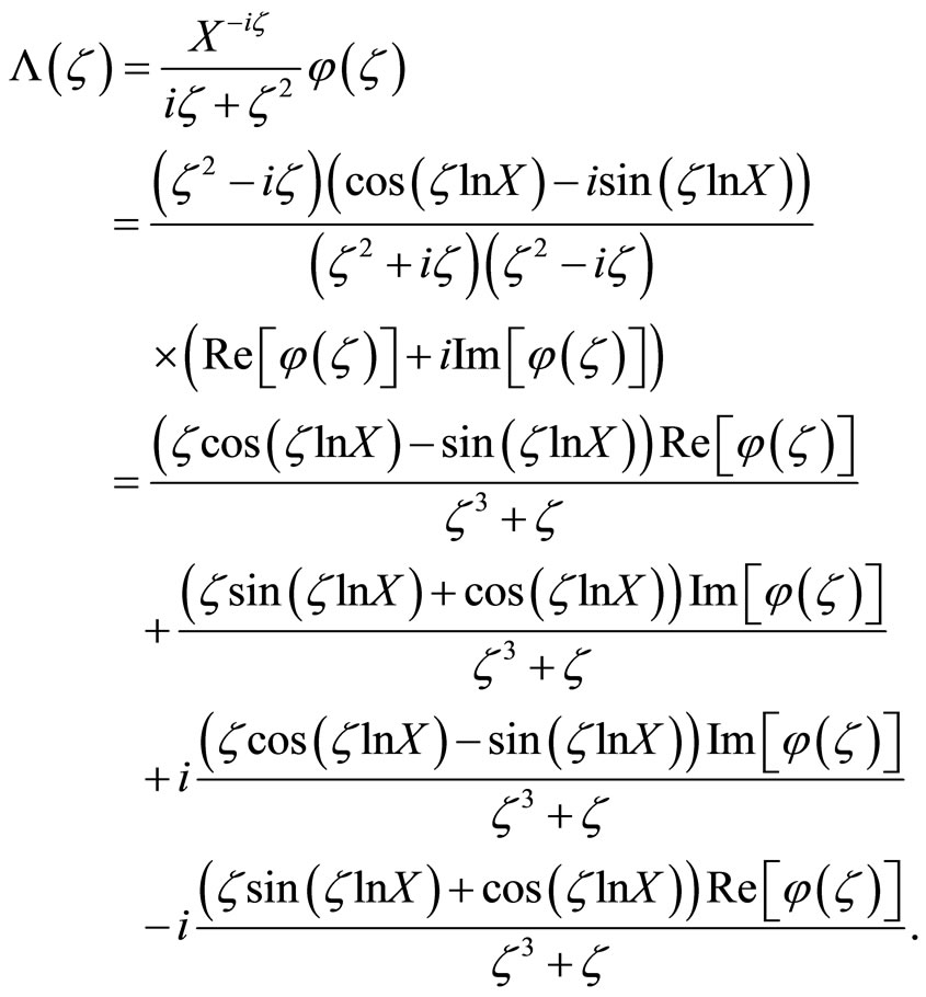
It then follows from the properties of trigonometric functions and Lemma 1 that  and
and . Therefore, by applying properties of even and odd functions,
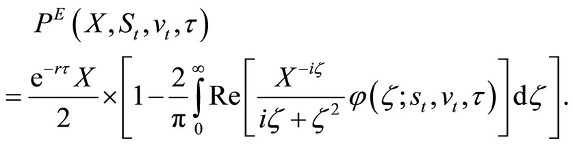 (10)
(10)
The oddness property of the imaginary part of  is not particularly surprising, since the imaginary part must integrate out to zero in order for
  in Equation (9) to be real-valued. However, the evenness property of the real part of
  is not immediately obvious. It allows for a reduction of the domain of integration, as Equation (10) shows.
Finally, let  denote the current value of a European-style call with a strike price X, given the stock’s price
 , volatility
  and time to expiration
  The call is allowed to be exercised on date T when its value will be
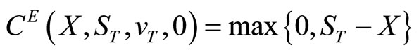 . By a put-call parity relationship for European-style options (Merton, 1973 [17]), which holds regardless of specific stock price dynamics,
 where
where  can be obtained using Equation (10).
5. Numerical Investigation
Equations (9) and (10) require numerical integration to calculate option values in practice. Intuitively, reducing the domain of integration in Equation (10) should allow for an increase in computational speed without a loss in precision. To assess actual performance of the two option value formulas, I conduct a numerical exercise. Namely, I calculate large series of put option values by applying both Equation (9) and Equation (10), and record the total computation time in each case. Parameter values used in the exercise are listed in Table 1 and correspond to calibrated values for the dynamics of the S & P 100 Index in July 2004 (Zhylyevskyy, 2010 [7]).3 Series of put options are generated by varying the underlying price  from 450 to 550 and the strike price X from 350 to 650. All options have a duration of three months. Numerical integration is implemented using the Gauss-Kronrod quadrature method (Press et al., 2001 [18]).
Table 2 reports the ratio of time needed to calculate all option values in series comprising 100, 10,000, and 1,000,000 options, using Equation (9) relative to Equation (10). As can be seen, by applying Equation (10) instead of Equation (9), the computation time can be cut almost in half. This outcome is expected since the integration in Equation (9) is conducted over the entire real line, while in Equation (10) it is only performed over the nonnegative domain. Most likely, since a small fixed cost of calling the integration routine is borne regardless of the region of integration, the computation speed increases by slightly less than twice overall.
The results of the numerical exercise indicate a computational advantage of Equation (10). This option value formula can help to reduce the cost of computationally intensive tasks that require evaluating multiple European-style derivative securities under Heston’s dynamics, such as in the cases of calibrating model parameters and calculating American-style option values by the compound-option scheme of Geske and Johnson (1984) [8].
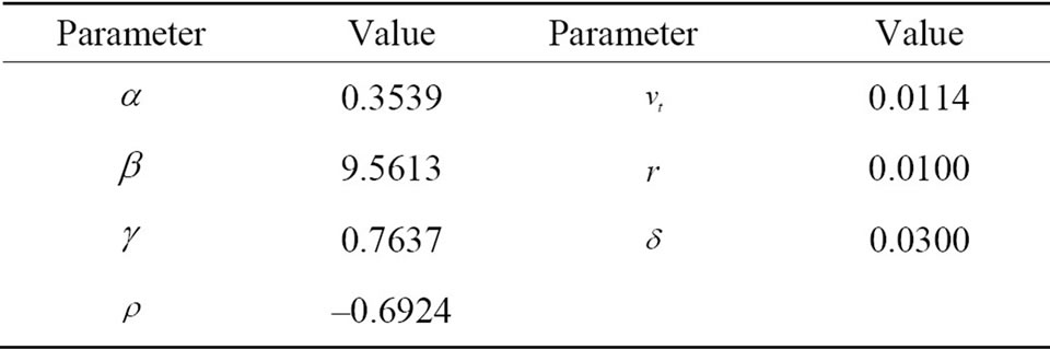
Table 1. Parameter values in numerical exercise.
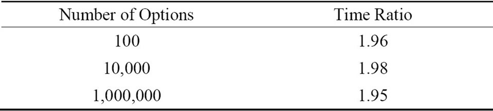
Table 2. Relative performance of option value formulas.
6. Conclusion
Efficient pricing of European-style derivatives under the stochastic volatility dynamics of Heston’s model has practical relevance, due to the model’s popularity. This paper utilizes a standard transform approach based on inverting the characteristic function of the log-price, and exploits the function’s symmetry in order to derive a computationally efficient formula for the value of a European-style put. The value of a call option is obtained using the parity relationship. The computational advantage of the formula stems from reducing the domain of integration in the inversion procedure, and is illustrated numerically. The method can help to mitigate the time cost of algorithms that require repeated evaluation of European-style options under Heston’s dynamics.
Appendix
The conditional characteristic function of the state vector  is
is
where complex-valued functions  and
and  are defined below.
In particular, if 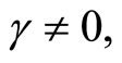
 and
and
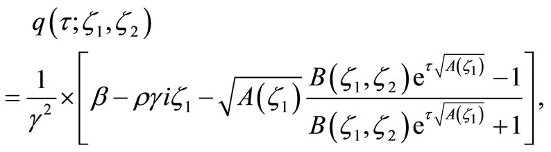
where

and
The case of  is not particularly interesting because it rules out stochastic volatility. Expressions for the functions p and q in that case and all derivations can be found in Zhylyevskyy (2010) [7].
NOTES
2Observe that the double integral is finite because

3The S & P 100 Index includes 100 leading stocks in the United States, which are components of the broader S & P 500 Composite Index and represent roughly 45% of the equity market capitalization.