Wrapped Skew Laplace Distribution on Integers:A New Probability Model for Circular Data ()
1. Introduction
Circular data arise in various ways. Two of the most common correspond to circular measuring instruments, the compass and the clock. Data measured by compass usually include wind directions, the direction and orientations of birds and animals, ocean current directions, and orientation of geological phenomena like rock cores and fractures. Data measured by clock includes times of arrival of patients at a hospital emergency room, incidences of a disease throughout the year, where the calendar is regarded as a one-year clock. Circular or directional data also arise in many scientific fields, such as Biology, Geology, Meteorology, Physics, Psychology, Medicine and Astronomy [1].
Study on directional data can be dated back to the 18th century. In 1734 Daniel Bernoulli proposed to use the resultant length of normal vectors to test for uniformity of unit vectors on the sphere [2]. In 1918 von Mises introduced a distribution on the circle by using characterization analogous to the Gauss characterization of the normal distribution on a line [2]. Later, interest was renewed in spherical and circular data by [3-5].
Circular distributions play an important role in modeling directional data which arise in various fields. In recent years, several new unimodal circular distributions capable of modeling symmetry as well as asymmetry have been proposed. These include, the wrapped versions of skew normal [6], exponential [7] and Laplace [8].
Wrapped distributions provide a rich and useful class of models for circular data.
The special cases of the wrapped normal, wrapped Poisson, wrapped Cauchy are discussed in [9]. We give a brief description of circular distribution in Section 2. In Section 3 we introduce and study Wrapped Discrete Skew Laplace Distribution. Section 4 deals with the estimation of the parameters using the method of moments.
2. Circular Distributions
A circular distribution is a probability distribution whose total probability is concentrated on the circumference of a circle of unit radius. Since each point on the circumference represents a direction, it is a way of assigning probabilities to different directions or defining a directional distribution. The range of a circular random variable Θ measured in radians, may be taken to be  or
or .
.
Circular distributions are of two types: they may be discrete - assigning probability masses only to a countable number of directions, or may be absolutely continuous. In the latter case, the probability density function  exists and has the following basic properties.
1) 
2) 
3) , for any integer k. That is
  is periodic with period
 .
.
Wrapped Distributions
One of the common methods to analyze circular data is known as wrapping approach [10]. In this approach, given a known distribution on the real line, we wrap it around the circumference of a circle with unit radius. Technically this means that if X is a random variable on the real line with distribution function , the random variable
 of the wrapped distribution is defined by
 (1)
(1)
and the distribution function of  is given by
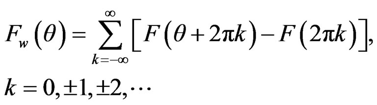 (2)
(2)
By this approach, we are accumulating probability over all the overlapping points  So if
So if  represents a circular density and
  the density of the real valued random variable, we have
 (3)
(3)
By this technique, both discrete and continuous wrapped distributions may be constructed. In particular, if X has a distribution concentrated on the points
 ,
,  and m is an integer, the probability function of
  is given by
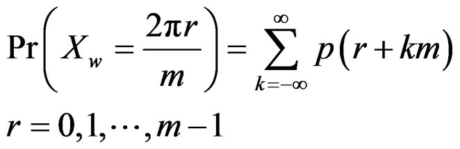 (4)
(4)
where “p” is the probability function of the random variable X.
3. Wrapped Discrete Skew Laplace Distribution
3.1. Discrete Skew Laplace Distribution
Discrete Laplace distribution was introduced by [11] following [12], who defined a discrete analogue of the normal distribution. The probability mass function of a general Discrete Normal random variable Y can be written in the form
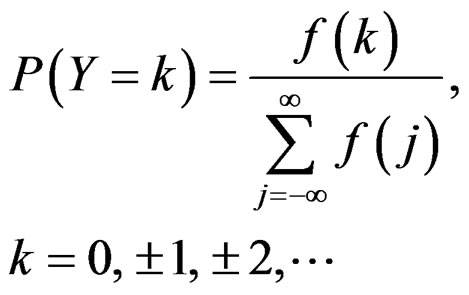 . (5)
. (5)
where “f” is the probability density function of a normal distribution with mean µ and variance  [13].
[13].
Using Equation (5), for any continuous random variable X on R, we can define a discrete random variable Y that has integer support on Z. When the skew Laplace density
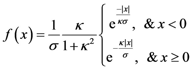 (6)
(6)
where,  , are inserted into Equation (5), the probability mass function of the resulting discrete distribution takes an explicit form in terms of the parameters p* =
 and
and .
.
Definition 3.1 A random variable Y has a discrete skew Laplace distribution with parameters 
and  denoted by DSL
 , if
, if
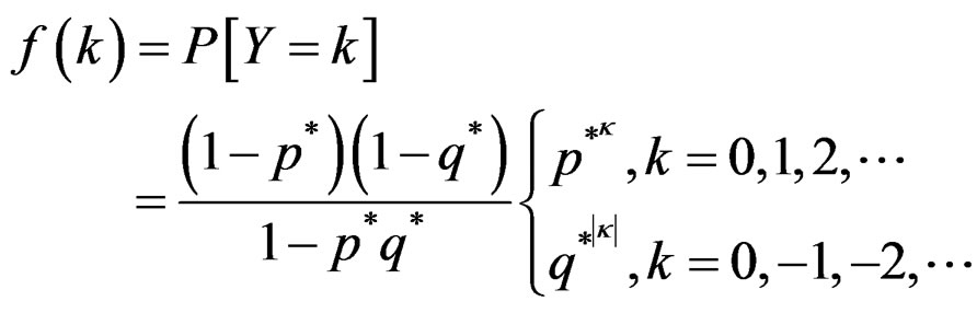 (7)
(7)
The characteristic function of Y is given by
 (8)
(8)
In this paper, we study the probability distribution obtained by wrapping discrete skew Laplace distribution on  around a unit circle.
As we know, reduction modulo 2π wraps the line onto the circle, reduction modulo 2πm (if m is a positive integer) wraps the integers onto the group of  root of 1, regarded as a subgroup of the circle. That is, if X is a random variable on the integers, then Θ, defined by
is a random variable on the lattice ,
, on the circle. The probability function of Θ is given by Equation (4).
In particular, if X has a discrete skew Laplace distribution with parameters  and
and , then the probability distribution of the wrapped random variable
  is given by
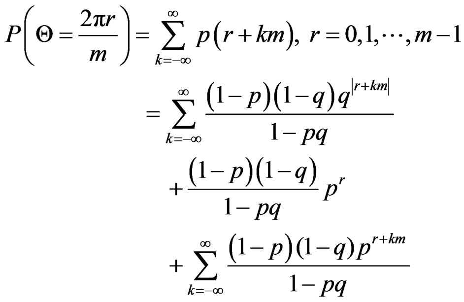
where  and
and
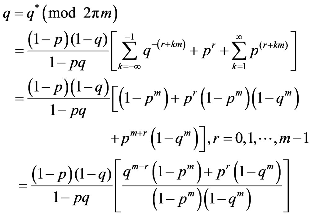 (9)
(9)
for  and
and
Again, we have
Hence  represents a probability distribution.
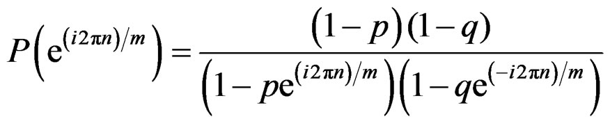
Definition 3.2 An angular random variable “Θ” is said to follow wrapped skew Laplace distribution on integers with parameters p, q and m if its probability mass function is given by
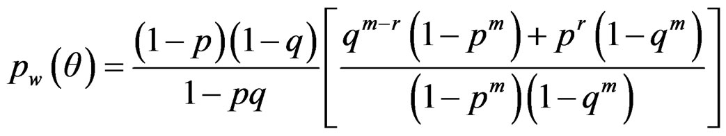 (10)
(10)
 and we denote it by WDSL
 .
.
Following are the graphs of wrapped discrete skew Laplace distribution for various values of κ, σ and m. In Figure 1, the graph of the pdf of wrapped discrete skew Laplace distribution for κ = 0.25, σ = 1 and for m = 5, 10, 20, 30, 40, 50 and 100 are given.
In Figure 2, the graph of the pdf of wrapped discrete skew Laplace distribution for κ = 0.5, σ = 1 and for m = 5, 10, 20, 30, 40, 50 and 100 are given. The graph of the pdf of wrapped discrete skew Laplace distribution for κ = 0.25, σ = 1 and for m = 5, 10, 20, 30, 40, 50 and 100 are given in Figure 3.
3.2. Special Cases
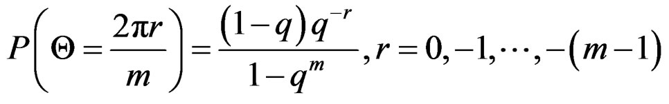
When either “p” or “q” converges to zero, we obtain the following two special cases:  with
with  is a wrapped geometric distribution with probability mass function
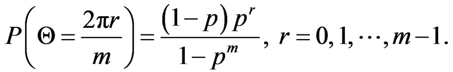 (11)
(11)
while  with
with  is a wrapped geometric distribution with probability mass function
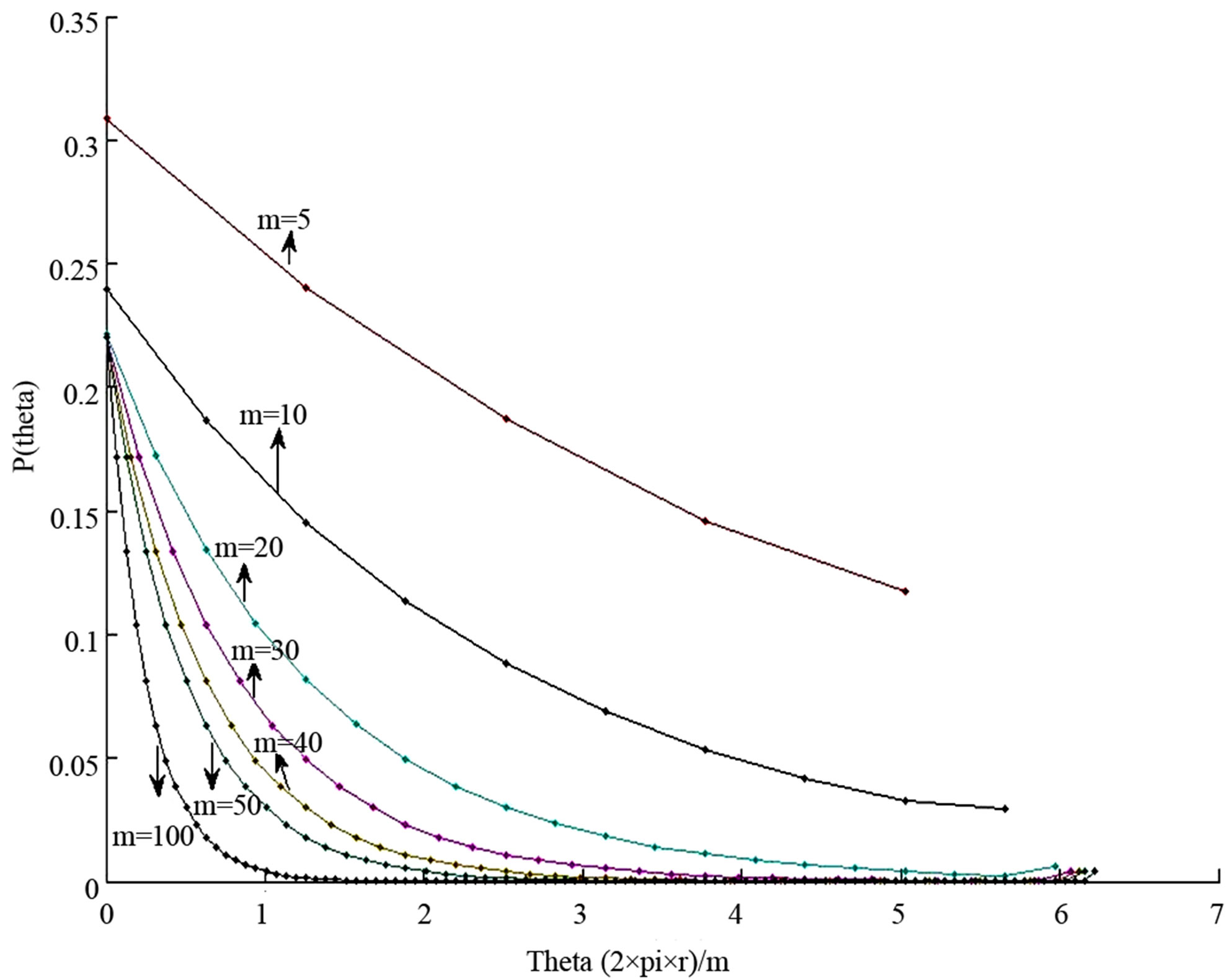
Figure 1. Wrapped discrete skewed Laplace distribution for ,
,  and for different values of “m”.
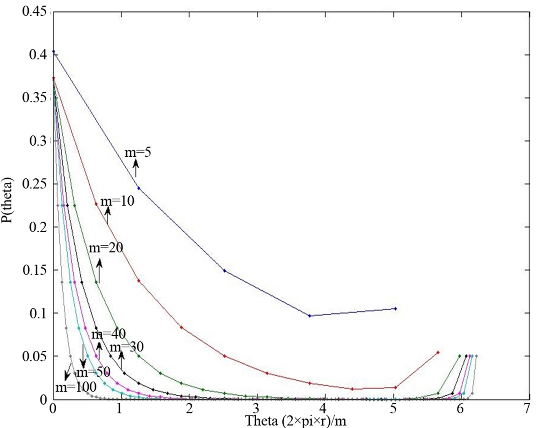
Figure 2. Wrapped discrete skewed Laplace distribution for ,
,  and for different values of “m”.

Figure 3. Wrapped discrete skewed Laplace distribution for ,
,  and for different values of “m”.
 . (12)
when p = q, we have
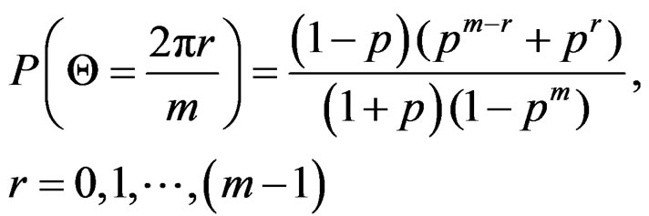 (13)
(13)
which is the probability mass function of wrapped discrete Laplace distribution.
3.3. Distribution Function of WDSL
The distribution function,  is given by
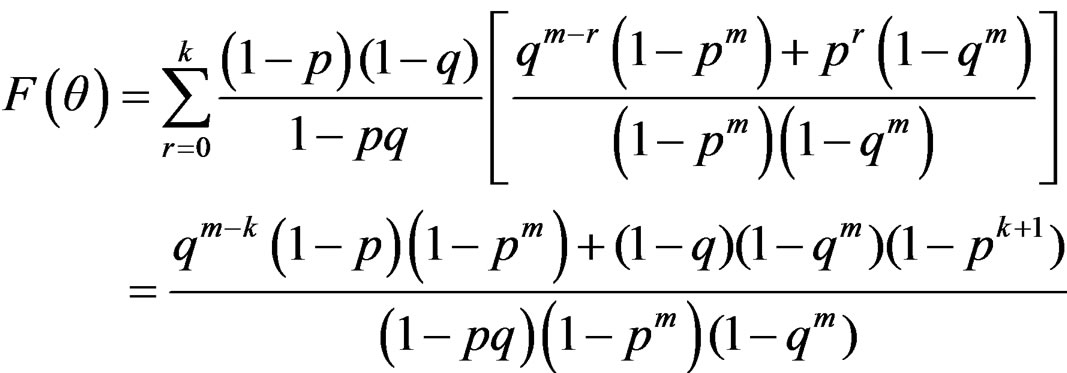 (14)
(14)
3.4. Probability Generating Function and Characteristic Function of WDSL
The probability generating function of WDSL is given by
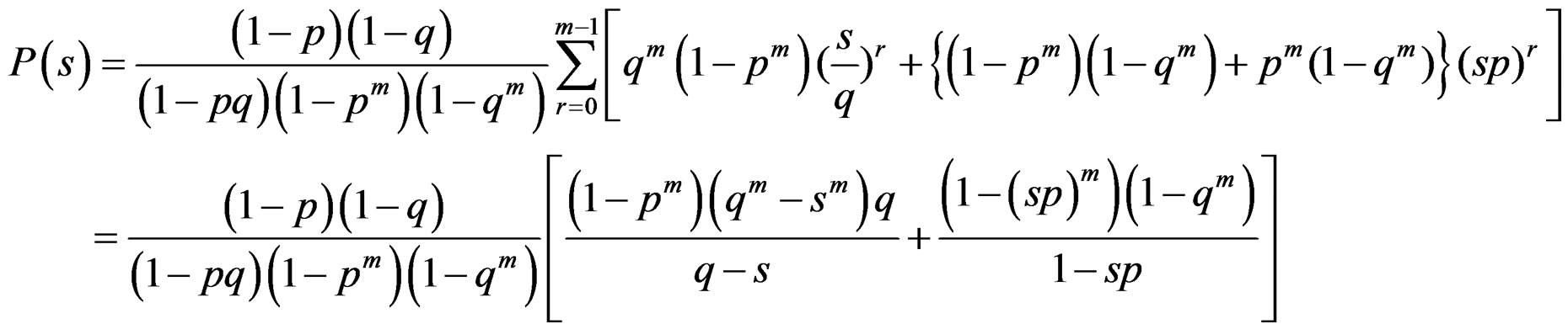 (15)
(15)
Also, we have .
.
when  we have
where 
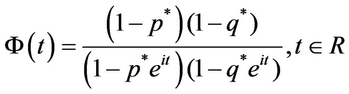
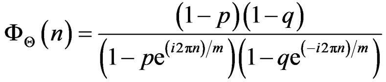
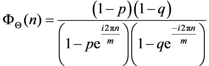
If  is the characteristic function of a linear random variable X, then the characteristic function of the wrapped random variable,
  is
is 

 [2]. Thus for the wrapped discrete skew Laplace distribution, we have
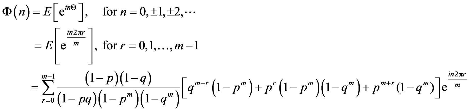 (16)
(16)
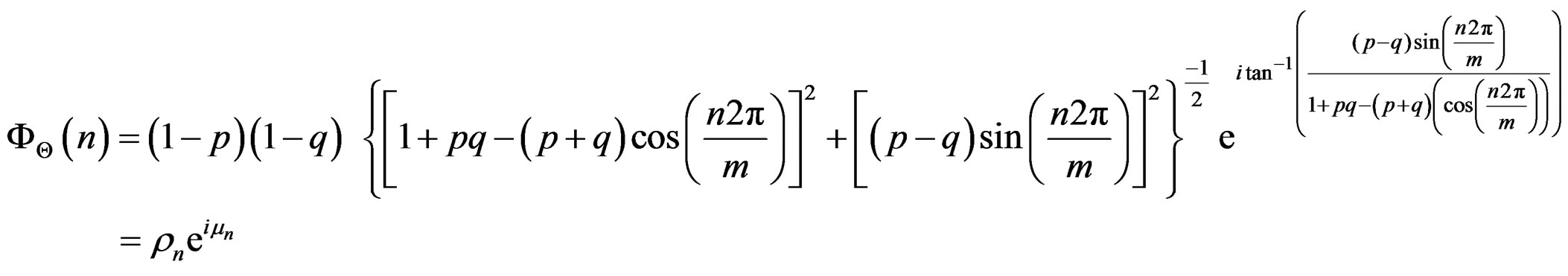
On simplification it reduces to
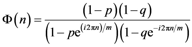 ,
,  (17)
(17)
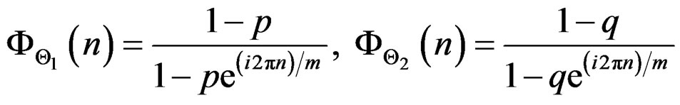
Again, we have
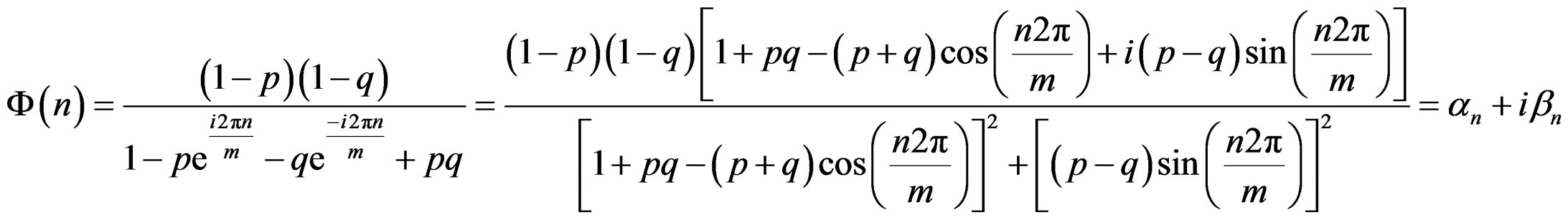
where

(18)
and
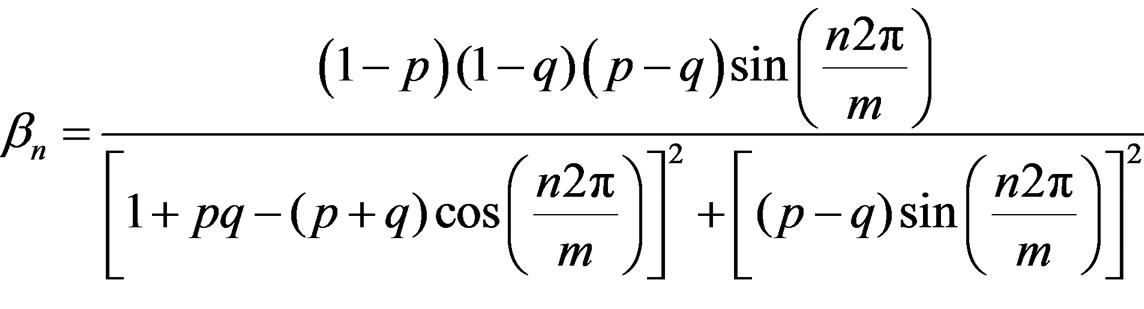
(19)
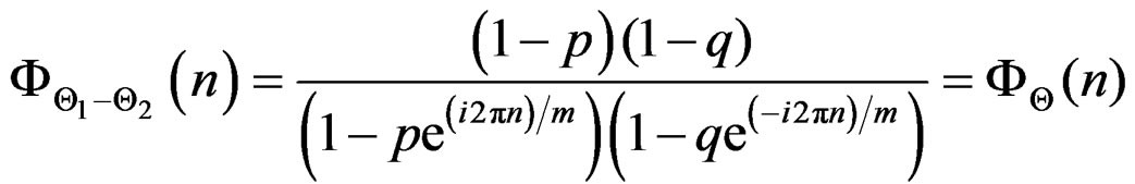
Proposition 3.1 If  then
then 
where  and
and  are two independently distributed wrapped geometric random variables with probability mass functions
 ,
,
Proof.
We have,

and
Therefore,
3.5. Infinite Divisibility
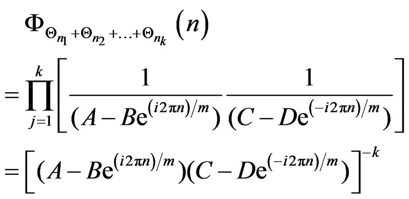
We know that the geometric distribution with probability mass function,  is infinitely divisible, so wrapped geometric distribution is infinitely divisible. Hence
  is infinitely divisible. By the well known factorisation properties of geometric law [14],
  admits a representation involving wrapped negative binomial distribution,
  where
where 
 .
.
Consider

where A, B, C, D > 0, A – B = C – D = 1 and ,
, 
Therefore,
3.6. Stability with Respect to Geometric Summation
Proposition 3.2. Let  be identically and independently distributed
  angular random variables, and let
  be a geometric random variable with probability mass function
 independent of
 . Then the angular random variable
 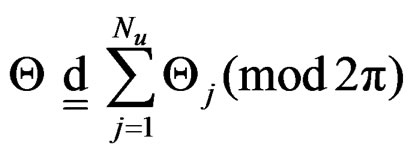 has the WDSL
 distribution with
Proof.
Let  be identically and independently distributed angular random variables following WDSL
 and
and  is a geometric random variable with mean
 . Conditioning on the distribution of
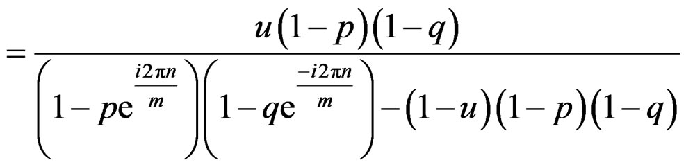
  we can write the characteristic function of the right hand side of the above equation as (Equation (20))
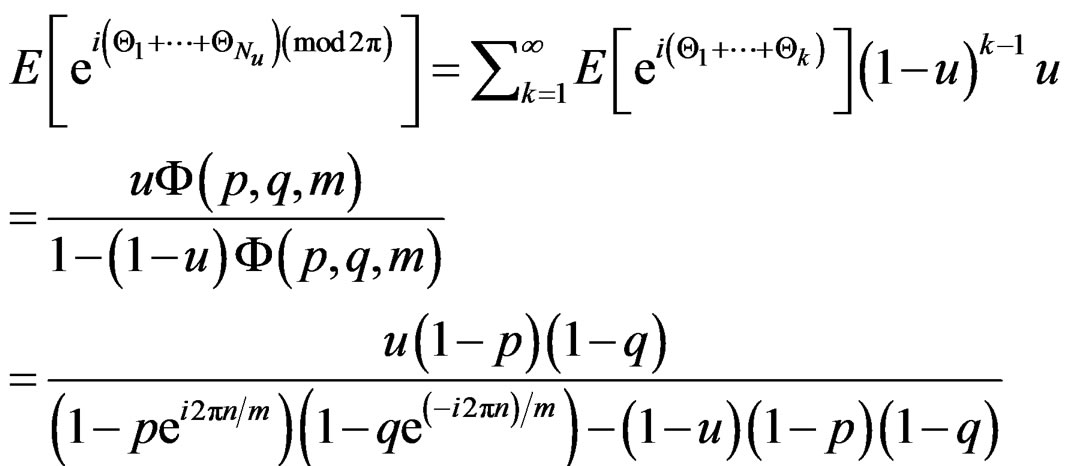 (20)
(20)
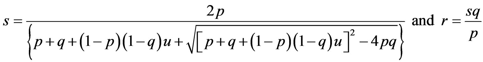
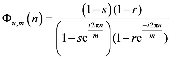
Now we show that the above function coincides with the characteristic function of  distribution with s and r as given above. Setting Equation (20) equal to
 , which is the characteristic function of
  distribution, produces the equation
 (21)
(21)
(22)
That is,

which should hold for each p, q. This will happen when the following two equations hold simultaneously.
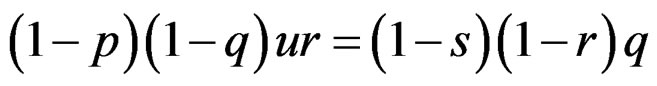 (23)
(23)
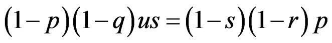 (24)
(24)
Dividing Equation (23) by Equation (24), we get
 Substituting the value of r in Equation (23) we get
 (25)
(25)
On simplification, Equation (25) reduces to
 (26)
(26)
That is, .
.
Since , and
, and  .
.
Therefore,  admits a unique solution in the interval
  and is given by
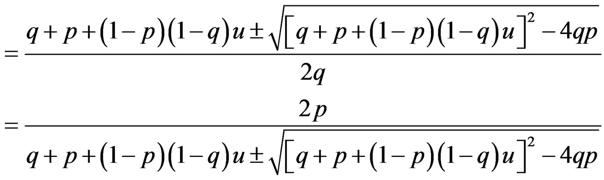 (27)
(27)
Remark 3.1. Wrapped discrete skew Laplace distribution is infinitely divisible since a circular random variable obtained by wrapping an infinitely divisible random variable is infinitely divisible by [1,11] .
3.7. Trigonometric Moments
The  trigonometric moment of the WDSL
is given by
The above expression can also be expressed in the form
where  is the
  th mean resultant length and
  is the
  th mean direction, for
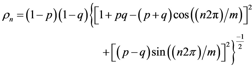 (28)
(28)
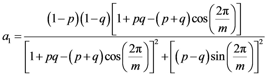
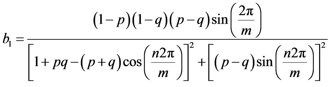
and
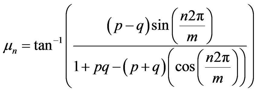 (29)
(29)
The length of the mean resultant vector,

and the mean direction, 
The circular variance,
The circular standard deviation,
The measure of skewness,
 where
where 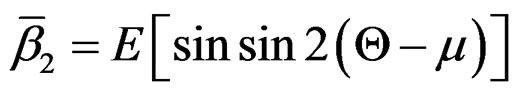
The measure of kurtosis,
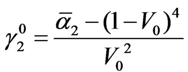 where
where 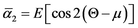
4. Estimation
Method of Moments
Let  be a random sample of size n taken from the WDSL
  distribution with parameters p, q, and m. Then the
  sample trigonometric moment about the zero direction,
 (30)
(30)
where
 (31)
(31)
and
 (32)
(32)
Corresponding population moment is  Equating the sample moments to the corresponding population moments, we get
  and
and  for
for . Thus, we have
 (33)
(33)
and
(34)
Using Equations (33)-(34) and for a fixed value of “m” we can find estimates for “p” and “q”.
We have,
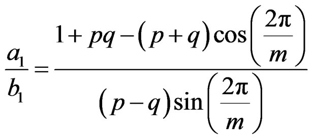
That is
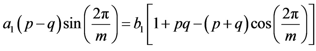
which gives
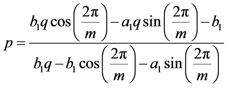 (35)
(35)
Substituting the value of “p” in terms of “q” in Equation (33) or in Equation (34) we will get an equation in “q” and solving that we can find the estimate of “q” and thus “p”.