LRS Bianchi Type-I Universe with Anisotropic Dark Energy in Lyra Geometry ()
The exact solutions of the Einstein field equations for dark energy (DE) in Locally Rotationally Symmetric (LRS) Bianchi type-I metric under the assumption on the anisotropy of the fluid are obtained for exponential volumetric expansion within the frame work of Lyra manifold for uniform and time varying displacement field. The isotropy of the fluid and space is examined.
1. Introduction
After the discovery that the cosmic expansion is accelerating [1-3] and the first cosmic microwave background (CMB) radiation observation of a flat universe [4], the current standard model of cosmology implies the existence of dark energy which accounts for about 70% of the total energetic content of the universe, which according to the observations is spatially flat [5]. The nature of the dark energy is still a mystery [6]. Several models have been proposed to explain dark energy [7-15]. An alternative consists of to consider a phenomenological decaying dark energy density with continuous creation of matter [15] or photons [16,17]. The dark energy might decay slowly in the course of the cosmic evolution and thus provide the source term for matter and radiation. Different such models have been discussed and strong constraints come from accurate measurements of the CMB. Although some authors [18] have suggested cosmological model with anisotropic and viscous dark energy in order to explain an anomalous cosmological observation in the cosmic microwave background (CMB) at the largest angles. The binary mixture of perfect fluid and dark energy was studied for Bianchi type-I and for Bianchi type-V [19] and [20] respectively. Akarsu et al. [21] have studied the Bianchi type-III with anisotropic dark energy.
Bianchi type models have been studied by several authors in an attempt to understand better the observed small amount of anisotropy in the universe. The same models have also been used to examine the role of certain anisotropic sources during the formation of the large-scale structures we see in the universe today. Some Bianchi cosmologies, for example, are natural hosts of large-scale magnetic fields and therefore, their study can shed light on the implications of cosmic magnetism for galaxy formation. The simplest Bianchi family that contains the flat FRW universe as a special case are the type-I space-times.
Lyra [22] proposed a modification of Riemannian geometry by introducing a gauge function into the structure-less manifold, as a result of which the cosmological constant arises naturally from the geometry. This bears a remarkable resemblance to Weyl’s [23] geometry. In subsequent investigations Sen [24] and Sen & Dunn [25] formulated a new scalar-tensor theory of gravitation and constructed an analog of the Einstein field equations based on Lyra’s geometry. Halford [26] has shown that the scalar-tensor treatment based on Lyra’s geometry predicts the same effects as in general relativity. Several authors studied cosmological models based on Lyra’s manifold with a constant displacement field vector . However, this restriction on the displacement field to be constant is only for convenience and there is no prior reason for it. Many authors studied the cosmological models with constant and time dependent displacement field [27-38]. Recently, the FRW cosmological model within the frame of Lyra geometry has been studied with variable Equation of state (EoS) parameter [39].
In the present paper, a spatially homogeneous and anisotropic LRS Bianchi type-I cosmological model with anisotropic dark energy in Lyra’s geometry for uniform and time varying displacement field has been studied. The geometrical and physical aspects of the model have been studied.
2. Metric and Field Equations
The LRS Bianchi type-I metric is given by
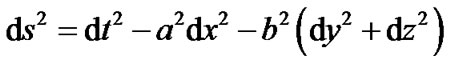 , (1)
, (1)
where the scale factors a and b are functions of cosmic time t only.
The energy-momentum tensor of anisotropic fluid is
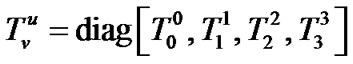 .
.
By parametrizing it, we get
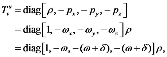 (2)
(2)
where is the energy density of the fluid;
 and
and  are the pressures and
  and
and  are the directional equation of state (EoS) parameters of the fluid.
Now, parametrizing the deviation from isotropy by setting , then introducing skewness parameter
  which is the deviation from
  on y and z axis. Here
  and
and  are not necessarily constants and can be functions of the cosmic time t.
The field equations in Lyra’s manifold as obtained by Sen [24] are  and
and 
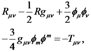 (3)
(3)
where  is the four velocity vector,
 is the displacement vector,
  is the Ricci tensor; R is the Ricci scalar,
 is the energy-momentum tensor .
In a co-moving coordinate system, above field Equations (3), for the anisotropic space-time (1), with Equations (2) yield
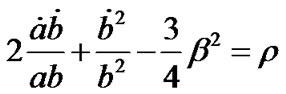 (4)
(4)
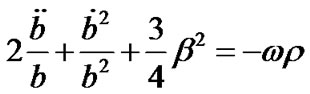 (5)
(5)
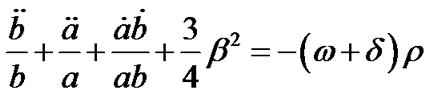 , (6)
, (6)
where the overhead dot (.) denote derivative with respect to the cosmic time t .
3. Isotropization and the Solution
The spatial volume is given by
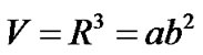 , (7)
, (7)
where  is the mean scale factor.
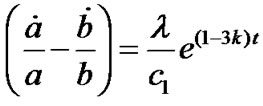
Subtracting Equation (5) from Equation (6), we get
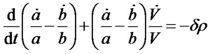 .
.
This on integrating gives
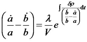 , (8)
, (8)
where  is constant of integration.
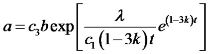
In order to solve the above Equation (8), we use the condition
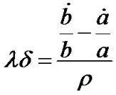 . (9)
. (9)
Using Equation (9) in the Equation (8), we obtain
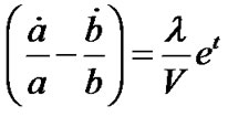 . (10)
To solve the system of equations completely we use law of variation for the Hubble parameter which yields the constant value of deceleration parameter proposed by [40] for FRW metric and then by [41] and [42] for Bianchi type space-times.
According to this law, the variation of the mean Hubble parameter for the metric (1) is given by
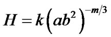 , (11)
where  and
and  are constants.
Here, in particular, we consider the model for  only. i.e. we consider the model for exponential expansion.
The directional Hubble parameters in the direction of x, y and z axis respectively for the LRS Bianchi type-I metric are
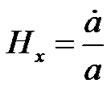 , and
, and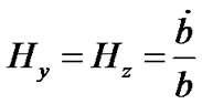 . (12)
The mean Hubble parameter is given as
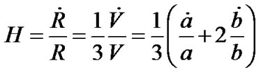 . (13)
The volumetric deceleration parameter is
 . (14)
On integrating, after Equations (11) and (13), we get
 for
for , (15)
where  is a positive constant of integration.
Using (11) with (15) for , we get
 (16)
(16)
Using Equations (15) and (7) in Equation (14) we get, constant values for the deceleration parameter for mean scale factor as:
 for
for , (17)
For this model  which implies the fastest rate of expansion of the universe. The deceleration parameter of the universe is in the range
  and the present day universe is undergoing accelerated expansion [2,3].
4. Model for Exponential Expansion i.e. for  (
( )
)
Using Equation (15) in the Equation (10), we get
 .
.
This on integrating gives
 , (18)
where  is a constant of integration.
Using Equation (18) in Equation (15), we get the value of scale factors as
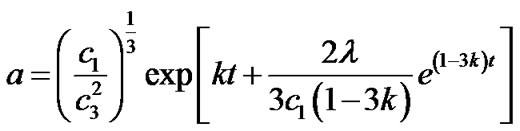 (19)
(19)
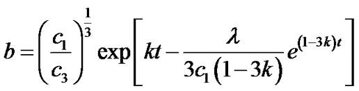 . (20)
The directional Hubble parameters are
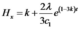 (21)
(21)
and
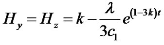 . (22)
The anisotropic parameter of the expansion  is defined as
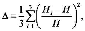
where  represents the directional Hubble parameters in the direction of x, y and z respectively.
Case (I): Uniform displacement field i.e. when , constant.
Here, we assume the vector displacement field  to be the time like constant vector
 , where
  is a constant.
The anisotropic parameter of the expansion ( ) is found as
 . (23)
The expansion scalar  is given by
 . (24)
The shear scalar  is given by
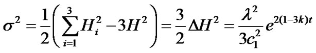 . (25)
Using Equations (21) and (22) in Equation (4), we obtain the energy density for the model as
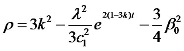 . (26)
Using Equations (21), (22) and (26) in Equation (9), we obtain the deviation parameter as
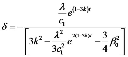 . (27)
Using Equations (21), (22), (26) and (27) in Equation (6), we obtain the deviation-free parameter as
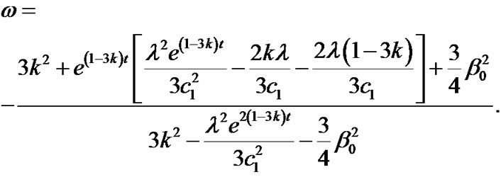 (28)
(28)
The anisotropy of the expansion ( ) is not promoted by the anisotropy of the fluid and decreases to null exponentially as t increases provided
 .
.
The space approaches to isotropy in this model since  as
as .
.
Also the spatial volume  and
and
 as
as  for
for .
.
Here  and
and  contribute to the energy density of the fluid
  negatively.
The energy density of the fluid , the deviation-free EoS parameter
  and the deviation parameter
  are dynamical.
For  and as
 , the anisotropic fluid isotropizes since
  and the model exhibits like phantom energy model having EoS parameter
 which is equivalent to
  provided that
 .
.
In this case (model), we get  as
as . i.e. for very very small positive value of
 , the model approaches [nearer to] the cosmological constant (
 ).
).
Also for , our model does not survive.
Case (II): Time varying displacement field i.e. when .
.
Here, we assume the vector displacement field  to be the time varying vector
 , where
 .
.
We consider  i.e.
i.e.
 . (29)
The anisotropic parameter of the expansion ( ) is found as
 . (30)
Using Equation (29) in the Equations (26), (27) and (28) we obtain, the energy density, deviation parameter and the deviation-free parameter for the model respectively as fallows:
 (31)
(31)
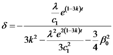 (32)
(32)
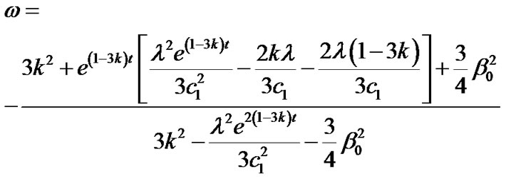 (33)
(33)
Here, the anisotropy of the expansion ( ) is not promoted by the anisotropy of the fluid and decreases to null exponentially as t increases provided
  .
.
The space approaches to isotropy in this model since  as
as .
.
The spatial volume  and
and 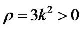 as
as  for
for .
.
Here  and
and  contribute to the energy density of the fluid
  negatively.
The energy density of the fluid , the deviation-free EoS parameter
  and the deviation parameter
  are dynamical.
For  and as
 , the anisotropic fluid isotropizes and mimics to the vacuum energy which is mathematically equivalent to the cosmological constant (
 ). i.e. we get
 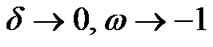 and
and  which matches with the result obtained by Akarsu et al. [21]. Also, in this case for
 , our model does not survive.
5. Conclusions
In case I and Case II, it is observed that the universe can approach to isotropy monotonically even in the presence of an anisotropic fluid in the model. The anisotropy of the fluid also isotropizes at later times and evolves into the well known cosmological constant in the model for exponential volumetric expansion. Also, for  our model does not survive. In case-I, the model evolves to the phantom energy and in case-II, it evolves to the cosmological constant (
 ). Thus, even if we observe an isotropic expansion in the present universe we still cannot rule out possibility of DE with an anisotropic EoS in Lyra geometry. Also, the role of displacement field
  plays a crucial role in the dynamics of the universe. Therefore, we cannot rule out the possibility of an anisotropic nature of the DE at least in the framework of Lyra geometry. These observations are worth to pay attention.
[1] J. A. S. Lima, “Thermodynamics of Decaying Vacuum Cosmologies,” Physical Review D, Vol. 54, No. 4, 1996, pp. 2571-2577. doi:10.1103/PhysRevD.54.2571
[2] S. Perlmutter, et al., “Measurements of Ω and Λ from 42 High-Redshift Supernovae,” The Astrophysical Journal, Vol. 517, No. 2, 1999, pp. 565-586. doi:10.1086/307221
[3] A. G. Reiss, et al., “Observational Evidence from Supernovae for an Accelerating Universe and a Cosmological Constant,” The Astrophysical Journal, Vol. 116, No. 3, 1998, pp. 1009-1038. doi:10.1086/300499
[4] P. de Bernardis, et al., “A Flat Universe from HighResolution Maps of the Cosmic Microwave Background Radiation,” Nature, Vol. 404, 2000, pp. 955-955. doi:10.1038/35010035
[5] D. N. Spergel, et al., “Three-Year Wilkinson Microwave Anisotropy Probe (WMAP) Observations: Implications for Cosmology,” The Astrophysical Journal Supplement Series, Vol. 170, No. 2, 2007, pp. 377-408. doi:10.1086/513700
[6] R. Caldwell and M. Kamionkowski, “The Physics of Cosmic Acceleration,” Annual Reviews: Nuclear and Particle Science, Vol. 59, 2009, pp. 397-429. doi:10.1146/annurev-nucl-010709-151330
[7] P. J. E. Peebles and B. Rathra, “The Cosmological Constant and Dark Energy,” Reviews of Modern Physics, Vol. 75, No. 32, 2003, pp. 559-606. doi:10.1103/RevModPhys.75.559
[8] T. Padmanabhan, “Cosmological Constant—The Weight of the Vacuum,” Physics Reports, Vol. 380, No. 5-6, 2003, pp. 235-320. doi:10.1016/S0370-1573(03)00120-0
[9] E. Tortora and M. Demianski, “Two Viable Quintessence Models of the Universe: Confrontation of Theoretical Predictions with Observational Data,” Astronomy & Astrophysics, Vol. 431, No. 1, 2005, pp. 27-44. doi:10.1051/0004-6361:20041508
[10] V. F. Cardone, et al., “Some Astrophysical Implications of Dark Matter and Gas Profiles in a New Galaxy Cluster Model,” Astronomy & Astrophysics, Vol. 429, No. 1, 2005, pp. 49-64. doi:10.1051/0004-6361:20040426
[11] R. R. Caldwell, “A Phantom Menace? Cosmological Consequences of a Dark Energy Component with Super-Negative Equation of State,” Physics Letters B, Vol. 545, No. 1-2, 2002, pp. 23-29. doi:10.1016/S0370-2693(02)02589-3
[12] P. J. E. Peebles and B. Rathra, “Cosmology with a TimeVariable Cosmological ‘Constant’,” Astrophysical Journal, Part 2 Letters, Vol. 325, No. 2, 1988, pp. L17-L20. doi:10.1086/185100
[13] B. Rathra and P. J. E. Peebles, “Cosmological Consequences of a Rolling Homogeneous Scalar Field,” Physical Reviews D, Vol. 37, No.12, 1988, pp. 3406-3427. doi:10.1103/PhysRevD.37.3406
[14] V. Sahni and A. A. Starobinsky, “The Case for a Positive Cosmological λ-Term,” International Journal of Modern Physics D, Vol. 9, No.4, 2000, pp. 373-443. doi:10.1142/S0218271800000542
[15] Y.-Z. Ma, “Variable Cosmological Constant Model: The Reconstruction Equations and Constraints from Current Observational Data,” Nuclear Physics B, Vol. 804, No. 1-2, 2008, pp. 262-285. doi:10.1016/j.nuclphysb.2008.06.019
[16] J. A. S. Lima, et al., “Is the Radiation Temperature-Redshift Relation of the Standard Cosmology in Accordance with the Data?” Monthly Notices of the Royal Astronomical Society, Vol. 312, No. 4, 2000, pp. 747-752. doi:10.1046/j.1365-8711.2000.03172.x
[17] J. A. S. Lima and J. S. Alcaniz, “Angular size in quintessence cosmology,” Astronomy & Astrophysics, Vol. 348, No. 1, 1999, pp. 1-5.
[18] T. Koivisto and D. F. Mota, “Accelerating Cosmologies with an Anisotropic Equation of State,” The Astrophysical Journal, Vol. 679, No. 1, 2008, pp. 1-5. doi:10.1086/587451
[19] B. Saha, “Anisotropic Cosmological Models with Perfect Fluid and Dark Energy,” Chinese Journal of Physics, Vol. 43, No. 6, 2005, pp. 1035-1043.
[20] T. Singh and R. Chaubey, “Bianchi Type-I, III, V, VIo and Kantowski-Sachs Universes in Creation-Field Cosmology,” Astrophysics and Space Science, Vol. 321, No. 1, 2009, pp. 5-18. doi:10.1007/s10509-009-9989-6
[21] O. Akarsu and C. B. Kilinc, “Bianchi Type III Models with Anisotropic Dark Energy,” Genenal Relativity and Gravitation, Vol. 42, No. 4, 2010, pp. 763-775. doi:10.1007/s10714-009-0878-7
[22] G. Lyra, “Über eine Modifikation der Riemannschen Geometrie,” Mathematische Zeitschrift, Vol. 54, No. 1, 1951, pp. 52-64. doi:10.1007/BF01175135
[23] H. Weyl, “Reine Infinitesimalgeometrie,” Mathematische Zeitschrift, Vol. 2, No. 3-4, 1918, pp. 384-411.
[24] D. K. Sen, “A Static Cosmological Model,” Zeitschrift für Physik A Hadrons and Nuclei, Vol. 149, No. 3, 1957, pp. 311-323.
[25] D. K. Sen and K. A. Dunn, “A Scalar-Tensor Theory of Gravitation in a Modified Riemannian Manifold,” Journal of Mathematical Physics, Vol. 12, No. 4, 1971, pp. 578-287. doi:10.1063/1.1665623
[26] W. D. Halford, “Scalar-Tensor Theory of Gravitation in a Lyra Manifold,” Journal of Mathematical Physics, Vol. 13, No. 11, 1972, pp. 1399-1405. doi:10.1063/1.1665894
[27] M. S. Berman and F. Gomide, “Cosmological Models with Constant Deceleration Parameter,” General Relativity and Gravitation, Vol. 20, No. 2, 1988, pp. 191-198. doi:10.1007/BF00759327
[28] W. D. Halford, “Cosmological Theory Based on Lyra’s Geometry,” Australian Journal of Physics, Vol. 23, No. 4, 1970, pp. 863-869.
[29] D. K. Sen and J. R. Vanstone, “On Weyl and Lyra Manifolds,” Journal of Mathematical Physics, Vol. 13, No. 7 1972, pp. 990-994. doi:10.1063/1.1666099
[30] K. S. Bhamra, “A Cosmological Model of Class One in Lyra’s Manifold,” Australian Journal of Physics, Vol. 27, No. 5, 1974, pp. 541-547.
[31] T. M. Karade and S. M. Borikar, “Thermodynamic Equilibrium of a Gravitating Sphere in Lyra’s Geometry,” General Relativity and Gravitation, Vol. 9, No. 5, 1978, pp. 431-436. doi:10.1007/BF00759843
[32] D. R. K. Reddy and R. Venkateswarlu, “Birkhoff-Type Theorem in the Scale-Covariant Theory of Gravitation,” Astronomy & Astrophysics, Vol. 136, No. 1, 1987, pp. 191- 194. doi:10.1007/BF00661267
[33] H. Soleng, “Cosmologies Based on Lyra’s Geometry,” General Relativity and Gravitation, Vol. 19, No. 12, 1987, pp. 1213-1216. doi:10.1007/BF00759100
[34] T. Singh and G. Singh, “Bianchi Type-I Cosmological Models in Lyra’s Geometry,” Journal of Mathematical Physics, Vol. 32, No. 9, 1991, pp. 2456-2459. doi:10.1063/1.529495
[35] G. Singh and K. Desikan, “A New Class of Cosmological Models in Lyra Geometry,” Pramana: Physics and Astronomy, Vol. 49, No. 2, 1997, pp. 205-212. doi:10.1007/BF02845856
[36] F. Rahaman, “A Study of an Inhomogeneous Bianchi-I Model in Lyra Geometry,” Astrophysics and Space Science, Vol. 281, No. 3, 2002, pp. 595-600. doi:10.1023/A:1015819414071
[37] F. Rahaman, N. Begum and B. C. Bhui, “Cosmological Models with Negative Constant Deceleration Parameter in Lyra Geometry,” Astrophysics and Space Science, Vol. 299, No. 3, 2005, pp. 211-218. doi:10.1007/s10509-005-5943-4
[38] A. Pradhan, V. K. Yadav and I. Chakrabarty, “Bulk Viscous Frw Cosmology in Lyra Geometry,” International Journal of Modern Physics, Vol. 10, No. 3, 2001, pp. 339-349. doi:10.1142/S0218271801000767
[39] C. P. Singh, “Early Cosmological Models in Lyra’s Geometry,” Astrophysics and Space Science, Vol. 275, No. 4, 2001, pp. 377-383. doi:10.1023/A:1002708316446
[40] C. P. Singh, “Bianchi Type-II Inflationary Models with Constant Deceleration Parameter In General Relativity,” Pramana: Physics and Astronomy, Vol. 68, No. 5, 2007, pp. 707-720.
[41] C. P. Singh, et al., “Bianchi Type-V Perfect Fluid SpaceTime Models in General Relativity,” Astrophysics and Space Science, Vol. 315, 2008, pp. 181-189. doi:10.1007/s10509-008-9811-x
[42] A. G. Riess, et al., “Type Ia Supernova Discoveries at z > 1 from the Hubble Space Telescope: Evidence for Past Deceleration and Constraints on Dark Energy Evolution,” The Astrophysical Journal, Vol. 607, No. 2, 2004, pp. 665-678. doi:10.1086/383612