An Approach to Detect Structural Development Defects in Object-Oriented Programs ()
1. Introduction
Object-oriented programming is a paradigm used by a significant number of developers in the design, development, and implementation of software systems. It facilitates the maintenance phase of developed applications. Unfortunately, this phase is increasingly jeopardized by developers introducing development defects that negatively impact software quality [1] . Poor maintenance hinders system evolution, the ease of changes that software engineers could make, program understanding, and increases the tendency for errors. In summary, poor maintenance leads to the deterioration of software quality [2] and reduces the lifespan of systems [3] . These anomalies, which are not bugs or technically incorrect codes and do not immediately disrupt program operation, indicate weaknesses in design and can slow development or increase the risk of bugs or failures in the future [4] . They are identifiable based on the taxonomy of detection approaches presented by Hadj-Kacem et al. [5] from four sources of information: structural, semantic, behavioral, and historical. Structural defects essentially refer to code structure that violates object-oriented design principles, such as modularity, encapsulation, data abstraction, etc. [6] . Blob and Long Method are two structural defects that align with this assertion and are widespread in source code.
They are classified according to several abstractions [4] [7] which we group into two categories: traditional heuristic approaches and machine learning-based approaches. Due to the challenges of finding threshold values for metric identification, the lack of consistency between different identification techniques, the subjectivity of developers in defining defects, and the difficulty of manually constructing optimal heuristics [8] , research has shifted towards machine learning [9] . These models are mathematical techniques that use historical data to automatically identify complex patterns and make informed and intelligent decisions [10] . However, this new paradigm is mainly built by learning models taken individually, putting aside the adage that there is strength in numbers and rarely takes into account the imbalance of data in the context of source codes [10] .
Knowing that pre-trained models have the ability to extract nuanced features and contextual information, they could enable better discrimination between minority and majority classes in the context of imbalanced datasets.
What machine learning method is suitable for imbalanced datasets in the context of structural development defect detection?
Our main objective is therefore to build a model based on ensemble learning whose basic estimator is composed of a pre-trained model having the capacity to contribute to the balance of classes and a classifier.
Underlying questions arise based on the above objective.
RQ1: What is the optimal number of base estimators for a model?
RQ2: Do pre-trained models alleviate class imbalance?
RQ3: Is an ensemble learning method using a pre-trained model for vector representations incorporating a deep learning classifier the state-of-the-art for ensemble methods?
To address these concerns, we organize this article as follows: In the second section, we present a literature review on detection approaches and on ensemble learning methods. Section 3 presents our approach. In Section 4, we present and discuss our results, and finally, we conclude the article.
2. Related Works
In the field of structural development defect detection approaches, several classifications have been defined [5] [11] [12] . In this work, we summarize the classification into two groups, as indicated by Yue et al. [13] : traditional heuristic approaches and those based on machine learning.
2.1. Traditional Heuristic Approaches
The process of heuristic approaches generally unfolds in two steps. A set of metrics associated or not with specific indicators on code instances is calculated, characterizing the considered defect. Then, thresholds are applied to these metrics [14] . Following this framework, Peldszus et al. [15] proposed a model that associates software metrics and various indicators of code smells to allow the system not to deteriorate as it evolves. However, the subjectivity of code smell indicators can render detection tools unusable in certain contexts.
Chen et al. [16] simultaneously implemented the Pysmell tool, whose detection strategy involved applying a set of metrics associated with parameterized thresholds to relevant code excerpts. Similarly, Hammad et al. [17] designed a plugin named JFly (Java Fly) integrated into the Eclipse environment based on a set of rules characterizing the defects to be detected, including software metrics associated with thresholds. All these approaches use threshold values, posing the recurring problem of the subjectivity of optimal choice.
Traditional heuristic approaches are increasingly abandoned in defect detection methods due, among other reasons, to the subjectivity in defining threshold values, steering research towards machine learning [9] .
2.2. Machine Learning-Based Approaches
Machine learning is a field of study in artificial intelligence that aims to give machines the ability to “learn” from data through mathematical models [18] . Two methods of using machine learning algorithms represent the state of the art in research.
2.2.1. Individual Model Cases
Hamdy et al. [19] experimented with two recurrent neural networks, LSTM (Long short term memory) and GRU (Gated recurrent unit), and a convolutional neural network CNN to detect blob. They concluded that neural networks outperform commonly used machine learning models like Naïve Bayes, Random Forests, and Decision Trees.
Although adding the lexical and syntactic features of the source code to the software metrics has provided a set of relevant information to the training data, these features do not take into account the semantics of the code.
Kacem et al. [20] conducted a study using a hybrid method, coupling an unsupervised learning phase using a deep autoencoder whose purpose is to transform code snippets into vector representations of reduced dimensions and supervised learning (artificial neural network ) to classify these codes based on their vector characterizations.
Sharma et al. [11] compared three types of models: Convolutional Neural Networks (CNN), Recurrent Neural Networks (RNN), and autoencoders with hidden layers composed of dense neural networks (DNN), CNN, and RNN. The authors used the open-source Tokenizer tool to generate vector representations of code.
In these two aforementioned works, the process of vector representation of code snippets does not take into account the context of the code, which defines its meaning.
To take into account the semantics of the source code, Kacem et al. [20] designed an approach that generates vector representations from abstract syntax trees from code excerpts used as input parameters for a variational autoencoder (VAE) whose produce semantic information through learning Finally a logistic regression classifier is applied to this semantic information to determine whether a code snippet is a defect or not. The limitation of this work lies in the procedure for extracting representative vectors from code snippets, which involves several steps, potentially making the entire system more comple.
In the search for relevant feature definitions, Škipina et al. [21] recommended the use of pre-trained models derived from natural language processing algorithms for source code in defining vector representations of code snippets, as opposed to metric extraction tools that take a considerable amount of time for extraction, become quickly obsolete due to the rapid evolution of language concepts, and yield inconsistent results, even for well-established code metrics. They established that the state-of-the-art in pre-trained models for vector representations in the context of code snippets is the CodeT5 model.
The use of machine learning algorithms requires transforming code snippets into vector representations. Several approaches are employed to define these representations. They range from the use of contextual and less generalizable metric extraction tools, tokenization methods that do not consider the semantic aspects of the code, vectorization from abstract syntax trees combined with machine learning, making the entire system complex, and pre-trained models. Advancements in natural language processing tasks, from which source code processing is derived through deep learning, have led researchers to utilize these methods.
2.2.2. Ensemble Learning Methods
Ensemble learning methods are meta-learning methods that combine multiple models to obtain a global and robust model. They are obtained either by using different learning algorithms, by using the same algorithm but with different parameters or initializations, or by using different training subsets with the same algorithm [22] . The most well-known ones are bagging, boosting, and stacking [23] .
Khleel et al. [10] combined the random oversampling technique SMOTE with five machine learning models, including an XGBoost ensemble algorithm, which achieved better accuracy with both balanced and unbalanced data. Similarly, Madeyski and Lewowski [24] evaluated the performance of seven learning algorithms and an ensemble learning method to detect four structural defects. The authors concluded that, overall, the Random Forests ensemble method exhibited better performance.
The interest of these studies lies in the predominance of ensemble learning methods over individual machine learning algorithms. However, for a more thorough evaluation, a comparison between ensemble learning methods would be appropriate.
Dewangan et al. [25] experimented with five ensemble learning techniques and two neural networks (Dense Neural Network and Convolutional Neural Network) to assess the impact of metrics on the detection of development defects In the preprocessing phase, the authors applied the SMOTE class balancing technique to balance each class in each dataset and showed, among other things, that ensemble methods combined with the Chi-square technique, a relevant feature extraction method, improve the performance of code smell detection.
Mamatha et al. [26] empirically validated the effect of homogeneous ensemble methods on the prediction performance of software defect detection models. They observed a significant improvement in model performance.
To validate the best data balancing technique, Liu et al. [8] experimented with 31 balancing methods to detect structural defects. The authors concluded that ensemble learning techniques like DeepForest substantially improved classifier performance.
Ensemble learning techniques have proven their effectiveness in detecting structural development defects. They mitigate the class imbalance problem in certain contexts and have become the state-of-the-art methods in machine learning. However, like any machine learning algorithm, they become ineffective when the extracted features are not relevant. To the best of our knowledge, there is no approach that combines pre-trained models for relevant feature definitions and ensemble learning methods for the detection of structural defects
3. Presentation of Our Approach
In this section, we describe the targeted defects, datasets, predictors, ensemble method defining our model, algorithm, experiment parameters, and performance metrics used to evaluate our model.
3.1. Targeted Development Defects
In this article, we choose to detect the anti-pattern Blob and the code smell Long Method. The selection of these defects is not arbitrary. Blob and Long Method are two widely prevalent structural defects in software. Code affected by these defects tends to have errors, negatively impacting software quality [2] . Given that Blob represents an anti-pattern and Long Method signifies a code smell, they can be considered representative of structural defects. Additionally, most existing datasets support these two development defects [27] .
3.2. Acquisition and Processing of Training Data
In the quest for development defect detection approaches, the lack of community-validated reference data poses a challenge in validating obtained results [2] . To address this gap in reference datasets, several datasets have been proposed [1] [2] [13] [28] [29] .
Lewowski and Madeyski [30] introduced MLCQ, an extensive industrial-type database annotated and validated by experienced experts.
The severity labeling of data, with a multitude of code instances, meaning a database containing both defect and non-defect instances, advocate for the MLCQ dataset. Consequently, we choose the MLCQ dataset based on the aforementioned considerations. We define two classes, expressed as [31] as follows:
where
is a code snippet at the class or method level.
In this study, we will use two reduced MLCQ datasets, one balanced and another imbalanced, to account for real proportions for a proper evaluation of our model. Table 1 and Table 2 provide the distributions of these two datasets.
3.3. Vector Representation and Class Imbalance Management
We employ the pre-trained CodeT5 model in the context of this work for generating code vector representations. This choice is based on its state-of-the-art
![]()
Table 2. Dataset containing long method.
performance, and it captures the semantic nuances necessary for detecting code smells [21] . Leveraging the pre-training of this model, we address the imbalance issue within our dataset.
3.4. Ensemble Learning Methods
The bagging model is formalized as follows: Let
be the initial sample, where
is a code snippet, and
. Let B be bootstrap samples of n observations:
,
.
Let
, where
is the model trained with bootstrap sample b, composed of the pre-trained model MOD_PRE followed by a DNN.
The ensemble model is defined as:
(1)
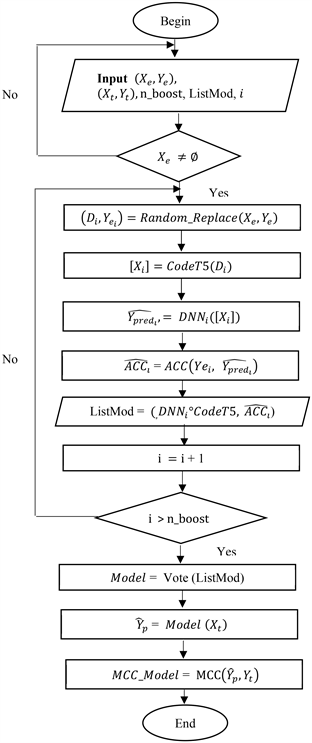
In our work, we experiment with CodeT5 as a pre-trained model and Roberta Classification Head for the DNN. The bagging technique is illustrated in the Figure 1.
3.5. Our Algorithm
3.5.1. Description of Our Algorithm
, and
are respectively the training and test data, ListMod is the container for the trained base estimators and corresponds to the number of base estimators to train. For each iteration i of , we select a sample
with replacement using the Random_replace function of the same size as the initial dataset
. We extract the features
from the code snippets using the pre-trained CodeT5 model, the first component of our model. This vector representation
is used as input to train our base estimator, which is the dense neural network
.
ACC is the function that evaluates the accuracy of the base estimator.Once all the base estimators are trained, each is associated with an accuracy. We obtain a list of pairs (
,
) that will be subjected to a Majority Voting procedure. This is the task of the vote function. It returns the final model that will be used for classification. Model evaluation is performed using the Matthews Correlation Coefficient (MCC) metric adapted for imbalanced data.We illustrate our algorithm with the diagram below.
3.5.2. Explanation of the Algorithm
and
are respectively the training and test data, ListMod is the container for the trained base estimators and n_boost corresponds to the number of base estimators to train. For each iteration i of n_boost, we select a sample
with replacement using the Random_replace function of the same size as the initial dataset
. We extract the features
from the code snippets using the pre-trained CodeT5 model, the first component of our model. This vector representation
is used as input to train our base estimator, which is the dense neural network
.
ACC is the function that evaluates the accuracy of the base estimator.
Once all the base estimators are trained, each is associated with an accuracy. We obtain a list of pairs (
,
) that will be subjected to a Majority Voting procedure. This is the task of the vote function. It returns the final model that will be used for classification. Model evaluation is performed using the Matthews Correlation Coefficient (MCC) metric adapted for imbalanced data.
3.6. Performance Evaluation Metrics
The usual model evaluation metrics that we will present subsequently are deduced from the confusion matrix defined by Table 3 for a binary classification.
Accuracy is the proportion of correctly predicted instances compared to all instances
(2)
Precision, also called positive predictive value, is the ratio of the number of true positives to the total number of positive predictions.
(3)
Recall or sensitivity or true positive rate is the proportion of positive instances actually predicted by the model among all truly positive instances
(4)
The F1-score is the harmonic mean of precision and recall
(5)
Mattheus Correlation Coefficient (MCC) measures the quality of a classification by comparing the model's predictions with the true class labels. It is particularly
![]()
Table 3. Confusion matrix for binary classification.
useful in scenarios where classes are unbalanced [32] .
(6)
4. Results and Discussion
4.1. Results
This section presents the results of our experiments in accordance with our research questions. In section 4.1.1, we will evaluate the impact of the number of base estimators in ensemble methods. Section 4.1.2 will justify the necessity or otherwise of class balancing through additional techniques. Section 4.1.3 will compare our method to RandomForest, and finally, section 3.4.2 will discuss our results.
4.1.1. Evaluation of the Number of Base Estimators in Ensemble Models
To better understand the impact of the number of base estimators in ensemble methods, we compare our model and RandomForest by varying the number of base estimators on two types of datasets. One balanced and the other imbalanced. Table 4 and Table 5, depicted by Figure 2 and Figure 3, respectively, show a comparison of the average accuracies between our model and RandomForest on
![]()
Table 4. Comparative table of average Accuracies between our model and RandomForest in the detection of Blob on the balanced dataset.
![]()
Figure 2. Comparison of accuracies in Blob detection on the balanced dataset.
![]()
Table 5. Comparative table of average Accuracies between our model and RandomForest in the detection of LongMethod on the balanced dataset.
![]()
Figure 3. Comparison of accuracies in Blob detection on the balanced dataset.
![]()
Table 6. Comparative table of average MCCs between our model and RandomForest in the detection of LongMethod on the unbalanced dataset.
the balanced dataset. Meanwhile, Table 6 and Table 7, illustrated by Figure 4 and Figure 5, present the average MCCs between our model and RandomForest on the imbalanced dataset.
4.1.2. Class Balancing
Can the use of pre-trained models adjust to minority classes? To address this concern, we evaluated our model with and without the SMOTE technique. On average, we achieved 87% accuracy, whether we associated the SMOTE technique with our model or not, with a very slight increase of 3% in MCC in favor of the balancing technique in the first eight trials. These empirical results suggest the unnecessary use of balancing techniques when pre-trained models are components of the model.
![]()
Figure 4. Comparison of MCCs in LongMethod detection on the unbalanced dataset.
![]()
Table 7. Comparative table of average MCCs between our model and RandomForest in the detection of blob on the unbalanced dataset.
![]()
Figure 5. Comparison of MCCs in Blob detection on the unbalanced dataset.
4.1.3. Comparison of Our Model and RandomForest
Our approach is compared to that of [24] , specifically to the RandomForest algorithm, which showed better performance according to the authors. Our 20 experiments rely on 10 base estimators trained on imbalanced datasets. We aggregated precision and recall by the mean, F1-score using equation (5), and accuracy and MCC by the median.
We summarize the results obtained in Table 8 and Table 9 with the associated graphical representations in Figure 6 and Figure 7, respectively.
4.2. Discussion
We posed questions for which experiments were undertaken to empirically confirm or refute assertions.
RQ1: How many basic estimators are needed for an optimal model?
To determine this number, we compared our model to RandomForest by varying the number of estimators. We observed that for a number of estimators
![]()
Table 8. Evaluation of our model and RandomForest in the detection of Long Method.
![]()
Figure 6. Evaluation of our model and RandomForest in the detection of Long Method.
![]()
Table 9. Evaluation of our model and RandomForest in the detection of Blob.
![]()
Figure 7. Evaluation of our model and RandomForest in the detection of Blob.
less than or equal to 20 for balanced datasets with a maximum size of 140, our model performed well in terms of accuracy. However, when data classes became imbalanced with a maximum size of 600, the number of estimators allowed by our experimental conditions became less than or equal to 10. In this context, we observed that RandomForest better detects the Blob anti-pattern from 7 estimators, while our model becomes effective from 10 estimators in detecting the LongMethod. These results need verification for larger numbers of estimators and larger datasets. We observed that when the imbalance is significant, both models tend to overfit. This observation could be verified by reconsidering the data and base estimator sizes.
RQ2: Do pre-trained models mitigate class imbalance?
From the experiments, it is not necessary to use additional class balancing techniques when pre-trained models are used to transform code snippets into vector representations. However, the question remains open when the imbalance is significant. We only used 8 experiments, as we noted that beyond this point, the variation in accuracy became low. This observation needs further justification.
RQ3: Is an ensemble method using a pre-trained model for vector representations and incorporating a deep learning classifier the state of the art in ensemble methods?
Since we use an unbalanced set, the preferred metric is MCC.
In Blob detection, the median MCC of our method is almost 20% lower than that of RandomForest. The F1-score and other performance metrics confirm the predominance of RandomForest over our model (See graph 4). However, our model outperforms RandomForest in LongMethod detection with a median MCC equal to 0.53 compared to 0.42 for RandomForest (See graph 3). These results suggest that ensemble learning methods based on deep learning estimators are not inherently more dominant in defect detection. However, the work of [19] has shown that neural networks outperform non-deep learning methods. Our underperformance in Blob detection could be explained by the small size of our dataset, as neural networks typically perform better when trained on large datasets.
5. Conclusions
Structural defects have a negative impact on software quality, making software maintenance challenging. Existing approaches do not integrate pre-trained models, which have the ability to define vector representations that consider the code semantics, and neural networks, which are highly effective in classification tasks. Therefore, we designed a bagging approach with CodeT5 and a dense neural network as the base estimator to detect Blob and LongMethod. We aimed to determine the optimal number of base estimators, but due to hardware resource limitations, we couldn’t establish a threshold for the number of estimators. In this study, we demonstrated that pre-trained models could, to some extent, address the issue of class imbalance in data. We compared our model with RandomForest, a reference model. Our results suggested that the choice of methods for detecting structural defects depended on the type of defects. However, we can confirm, based on the work of [18] , that the size of the data used biased the results.
For future work, we will use larger datasets and a greater number of estimators to evaluate our model. We will also examine the complexity of our model to reduce execution time compared to RandomForest.