1. Introduction
Efficient algorithms for computing maximum flows in networks are important not only because they are applied directly to the analysis of traffic or communication networks, but also because they are often employed as subproblems in other general network problems. Fundamental algorithms for network flow were designed and efficient algorithms exist (Ahuja, Magnanti, & Orlin) [1] to solve different instances of this problem. A natural generalization of the maximum flow problem can be obtained by making the capacities of some arcs functions of a single parameter. The parametric maximum flow problem is to compute all maximum flows for every possible value of the parameter. For the parametric maximum flow problem with zero lower bounds and linear capacity functions of a single parameter, Hamacher and Foulds [2] investigated an approach for determining in each iteration an improvement of the flow defined on the whole interval of the parameter while for the same problem, Ruhe [3], [4] proposed a “piece-by-piece” approach. The partitioning type approach, which is presented in this paper, proposes an original algorithm for computing the maximum flow in networks with constant lower bounds and linear upper bound functions.
Partitioning technique in network has been, in the latest years, a more and more active research topic in both engineering and theoretical research. The reason why the problem under consideration is of genuine practical and theoretical interest lies in that graph partitioning applications are described on a wide variety of subjects as: data distribution in parallel-computing, VLSI circuit design, image processing, computer vision, route planning, air traffic control, mobile networks, social networks, etc. [5]. Unfortunately, graph partitioning is an NP-hard problem, and therefore all known algorithms for generating partitions merely return approximations to the optimal solution.
Further on, this paper is organized as follows; Section 2 presents the basic network flow terminology and results used in the rest of the paper. More specialized terminology is developed in later sections. In Section 3, we introduce the parametric maximum flow problem and Section 4 presents the partitioning algorithm for solving this problem. Finally, Section 5 gives an example of how the algorithm works on a network with linear upper bound functions of a single parameter. In the presentation to follow, some familiarities with flow algorithms are assumed and many details are omitted, since they are straight forward modifications of known results. Further details on notions and results presented in Section 2 can be found in the papers of Ahuja et al. [1] and Ciurea et al. [6,7].
2. Terminology and Preliminaries
Let  be a capacitated network with
  nodes and
  arcs,
arcs,  being the set of nodes i and
  being the set of arcs a, so that for every arc in
 ,
,  with
with . The upper bound function and the lower bound function are two nonnegative functions,
  and
and  associated with each arc
 . The network has two special nodes: a source node
  and a sink node
 . A flow is a function
  satisfying the next conditions:
 (1)
(1)
for some , where
  is referred to as the value of the flow
 . Any flow on a directed network satisfying the flow bound constraints:
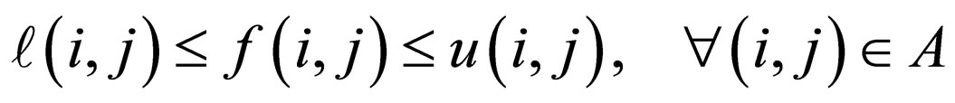 (2)
(2)
is referred to as a feasible flow. A cut is a partition of the node set  into two subsets
  and
and , denoted by
 . An arc
  with
with  and
and  is referred to as a forward arc of the cut while an arc
  with
with  and
and  as a backward arc of the cut. Let
  denote the set of forward arcs in the cut and
  denote the set of backward arcs. A cut
  is an
is an  cut if
  and
and . The maximum flow problem is to determine a flow
  for which
  is maximized. The maximum flow problem in a network can be solved in two phases: (1) establishing a feasible flow; (2) from a given feasible flow, establishing the maximum flow. For the first phase, see the algorithms presented in [1,7,8].
3. The Parametric Maximum Flow
The parametric flow problem consists in generalising the classic problem of flows in networks by transforming the upper bounds of some arcs  of the network
 in linear functions of a real parameter
 .
.
Definition 1. A directed network  for which the upper bounds
  of some arcs
  are functions of a real parameter
  is referred to as a parametric network and is denoted by
 .
.
For a parametric network , the parametric upper bound (capacity) function
  associates to each arc
  and for each of the parameter values
  in an interval
 , the real number
 , referred to as the upper bound of arc
 :
:
 (3)
(3)
where  is a real valued function associating to each arc
  the real number
 , referred to as the parametric part of the upper bound of the arc
 . The nonnegative value
  is the upper bound of the arc
  for
for , i.e.
 with
with . For the problem to be correctly formulated, the upper bound function of every arc
  must respect the condition
  for the entire interval of the parameter values, i.e.
  and
and . It follows that the parametric part of the upper bounds
  must satisfy the constraint:
 ,
, . The parametric flow value function
  associates to each of the nodes
  a real number
  referred to as the value of node
  for each of the parameter
  values.
Definition 2. A feasible flow in the parametric network  is called a parametric flow and it is a function
  satisfying the following constraints:
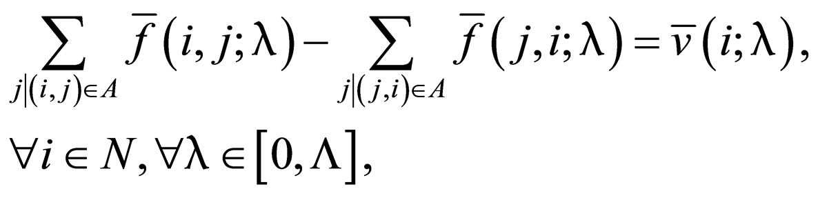 (4)
(4)
 (5)
(5)

The parametric maximum flow (PMF) problem is to compute all maximum flows for every possible value of :
:
 , (6)
, (6)
 (7)
(7)
 (8)
(8)
This problem looks like a classic maximum flow problem with the decisive difference that the variables  of this problem are piecewise linear functions instead of real numbers and that the upper bounds
 are linear functions instead of constants.
Definition 3. Let F be the set of piecewise linear functions  with
with . On the set F, an ordering relation is defined as follows:
 . (9)
. (9)
For any two piecewise linear functions  and
and , it is possible that neither the relation
  nor
nor  hold for the entire interval
  and consequently, the two functions may not necessarily be comparable. But it is always possible that a partitioning B:
 of the interval
  to be defined such as on every subinterval
 ,
, one of the two cases to hold:
  or
or , i.e. the two linear functions to become comparable. This means that the two functions have no crossing points within any subinterval
 , the only crossing points taking place for
 .
.
Proposition 1. For the parametric maximum flow problem, the subintervals ,
,  , of the parameter
  values can be defined so that a minimum
  cut in the non-parametric network
 , with
 , also to represent a minimum
  cut for all the parameter
  values within the subinterval
 .
.
Definition 4. A parametric  cut partitioningdenoted by
 ,
,  , is defined as a finite set of cuts
 ,
,  , together with a partitioning of the interval
  of the parameter in disjoints subintervals
 ,
,  , so that
 .
.
Definition 5. For the parametric maximum flow problem, the capacity  of a parametric
  cut partitioning is a linear function on every subinterval
 ,
,  , defined as:
 (10)
(10)
Definition 6. A parametric  cut partitioning
  with the subintervals
  assuring that every cut is a minimum cut
  within the subinterval
  is referred to as a parametric minimum
  cut and is denoted by
 ,
, .
.
Theorem 1. (Parametric max-flow min-cut theorem [9]) If there is a feasible flow in the parametric network , the value function
  of the parametric maximum flow
  from a source s to a sink t equals the capacity
  of the parametric minimum
  cut
cut ,
, .
.
Let  be a vector of feasible flow functions. Assuming that an arc
  carries a flow
 , the existing flow can be increased either by pushing the flow
  from node
  to node
  over the arc
 , or by pulling the flow
  from node
  to node
  along the arc
 . These flows are computed as differences between piecewise linear functions of
 .
.
Definition 7. For the parametric maximum flow problem, the parametric residual capacity  of any of the arcs
  with respect to a given parametric flow
  represents the maximum additional flow that can be sent from node
  to node
  over the arcs
  and
and  and is given by:
 .(11)
.(11)
Definition 8. The subintervals  where an augmentation of the flow
  is possible along the arc
  are defined as follows:
 (12)
(12)
Definition 9. Given a feasible flow  in the parametric network
 , the network denoted by
 with
with being the set consisting only of arcs with positive parametric residual capacities, is referred to as the parametric residual network with respect to the given flow
  for the parametric maximum flow problem.
If an arc  does not belong to
  then
then  is set.
Definition 10. A conditional augmenting directed path is denoted by  and is a directed path
  from the source s to the sink t in the parametric residual network
  with the restriction that:
 (13)
(13)
Definition 11. A partly conditional augmenting directed path is denoted by  and is a conditional augmenting directed path
  from the source s to node
 in the parametric residual network
 .
.
Definition 12. The parametric residual capacity of a conditional augmenting directed path  is the inner envelope of the parametric residual capacity functions
  for all arcs
  composing
  and for all parameter
  values in the subinterval
 :
:
 . (14)
Let  be the number of subintervals within the piecewise linear function
  maintains a constant slope. Since any conditional augmenting directed path
  is an elementary path, results that
 .
.
Theorem 2. (Conditional augmenting path theorem [9]) A flow  is a parametric maximum flow if and only if the parametric residual network
  contains no conditional augmenting directed path.
4. Partitioning Algorithm for the Parametric Maximum Flow Problem
The partitioning algorithm (PA) for the parametric maximum flow problem presented in this paper determines in each of its iterations an improvement of the flow over a subinterval of the parameter values generated by the partition induced by the first (in increasing order of their  values) of the breakpoints of the piecewise linear parametric residual capacity of the conditional augmenting directed paths
  in the parametric residual network. Since the parametric residual capacities for all the arcs in
 are linear functions of
 , the parametric residual capacity
  of any conditional augmenting directed path
  in the parametric residual network is a piecewise linear function of
  with
with  breakpoints.
In order to avoid working with piecewise linear functions, the algorithm works in several parametric residual networks defined for subintervals of the parameter values where the parametric residual capacities of all arcs remain linear functions. The parametric residual network defined for the subinterval
  of the parameter values is denoted by
 . Besides working with linear instead piecewise linear functions, another main advantage of our approach is that every augmenting directed path
  in a parametric residual network
  is also a conditional augmenting directed path
  in
in  for the subinterval
 for which the residual network
  is defined.
The first phase of finding a parametric maximum flow consists in establishing a feasible flow, if one exists, in a non-parametric network  obtained from the initial parametric network by only replacing the parametric upper bound functions with the non-parametric upper bounds:
  for
for and
and  for
for . After a feasible flow
  is established, the next step is to compute the parametric residual network
  for this feasible flow. For the non-parametric flow
 , the parametric residual capacities for every arc
  in
in  can be written as
 , where
  represents the slope of the parametric residual capacity function and
 is the value of the parametric residual capacity function computed for
 , i.e.
 .
.
The second phase of the algorithm starts with the parametric residual network , defined for the nonparametric feasible flow
 , which is also
 , i.e.
  and
and , since the residual capacities of all arcs are linear functions. The algorithm repeatedly finds shortest augmenting directed paths from the source node to the sink node in the parametric residual network and increases the flow in the original parametric network
  only in the subinterval
  which reflects in updating the parametric residual network
 . The parameter value
  is updated on each flow augmentation step so that the parametric residual capacities of all arcs not to have breakpoints within the interval
 . During its successive iterations, the algorithm maintains an ordered list
  of parameter values for which the parametric network is partitioned. This list is initialised as
  and is updated, each time the parametric residual network
 contains no conditional augmenting directed path, with a new
  value, representing the new lower limit of the subinterval of the parameter values for which a new parametric residual network
  is defined. At this point, the parametric maximum flow
  is computed for the subinterval
  and the algorithm goes on iterating within the next subinterval
 until the value
  is reached.
PARTITIONING ALGORITHM (PA);
1. BEGIN
2. compute a feasible flow  in network
 ;
;
3. compute the parametric residual network ;
;
4. ;
; ;
; ;
;
5. REPEAT
6. SSADP ;
;
7.  ;
;
8. UNTIL ( );
);
9. END.
In the k-th step of the partitioning algorithm (PA), the Successive Shortest Augmenting Directed Paths (SSADP) procedure computes the parametric residual network for the subinterval
 ,where the parametric residual capacities of all arcs can be written as
 ,with
,with and
and . As can be easily seen, the restriction
 ,
, is equivalent with
 .The SSADP procedure maintains a partly conditional augmenting directed path
  which is memorised in the predecessor vector
  and executes ADVANCE and RETREAT operations from the current node
  until the sink node
  is reached, i.e. the partly conditional augmenting directed path is transformed in a conditional augmenting directed path
 .
.
ADVANCE ; RETREAT
 ;
;
1. BEGIN 1. BEGIN
2.  ; 2.
; 2. ;
;
3.  ; 3. IF
  THEN
THEN ;
;
4. END; 4. END
From a current node , an ADVANCE operation will add the admissible arc
  to the partly conditional augmenting directed path while a RETREAT operation will eliminate the arc
  from it.
PROCEDURE SSADP ;
;
1. BEGIN
2. compute the parametrico residual network ;
;
3. compute the exact distance labels  in
in ;
;
4.  ;
; ;
; ;
; ;
; ;
;
5. WHILE  DO
DO
6. IF(exists an admissible arc ) THEN;
7. BEGIN
8. ADVANCE ;
;
9. IF  THEN
THEN
10. BEGIN
11. RC ;
;
12.  ;
;
13. END;
14. END;
15. ELSE RETREAT ;
;
16. compute the parametric maximum flow ;
;
17. add  to the list
 ;
;
18. END;
A call to Residual Capacity (RC) procedure will compute the parametric residual capacity  of the conditional augmenting directed path and will update the values
  and
and  according to the augmentation of the flow. After initializing
 and
and in order to assure that the parametric residual capacity
 remains a linear function without breakpoints in the subinterval
 , the slope
  of the parametric residual capacity
  is compared with the slopes
 of the parametric residual capacities of all the arcs
 .
.
If the condition  holds for an arc
 , it means that the linear functions
  and
and  have a crossing point for a parameter value
  and, consequently, the parametric residual capacity
  would have a breakpoint for
 .
.
If , i.e. the breakpoint is placed within the subinterval
 , the upper limit
  will be replaced with the new parameter value
 . Then, the parametric residual capacity
  will be subtracted from the parametric residual capacities of all arcs
  and added to those of the arcs
 , for all the parameter values in the new subinterval
 . As soon as
  contains no conditional augmenting directed paths, the parametric maximum flow
  is computed for the subinterval
  and the value
 is added to the list
 . Then the current value
  of the counter is incremented and, if the condition
  is not reached yet, the algorithm reiterates for the next subinterval
 . Otherwise, if
  equals
 , the whole interval of the parameter has been completed and the algorithm stops. For each of the subintervals
 ,
,  the parametric maximum flow is computed as
 .
.
PROCEDURE RC ;
;
1. BEGIN
2. compute  based on predecessor vector
 ;
;
3.  ;
;
4.  ;
;
5.  ;
;
6. WHILE  DO
DO
7. BEGIN
8. IF  THEN
THEN
9. BEGIN
10.  ;
;
11. IF  THEN
THEN ;
;
12. END;
13.  ;
; ;
;
14.  ;
; ;
;
15.  ;
;
16. END;
17. END;
Theorem 3. The Successive Shortest Augmenting Directed Paths (SSADP) procedure correctly computes a parametric maximum flow in the parametric network for the parameter
  values in the subinterval
 .
.
Proof. Since procedure SSADP works in the parametric residual network  for which the parametric residual capacities
  of all arcs
  and the parametric residual capacity
  of any of the augmenting directed paths
 , are linear functions without crossing points within the subinterval
 , the correctness of the procedure results from the correctness of the shortest augmenting directed path algorithm for the non-parametric case.
Theorem 4. The Residual Capacity (RC) procedure correctly computes the parametric residual capacity
 of a conditional augmenting directed path
  in the parametric residual network
  for the parameter
  values in the subinterval
 .
.
Proof. As the parametric residual capacity  is the inner envelope of the parametric residual capacity functions
  of all arcs composing the conditional augmenting directed path and since these parametric residual capacities are linear functions for the entire subinterval
 , the proof results from choosing the minimum possible values (lines 3 and 4 of procedure RC) for
  and for the corresponding
 , as well as from continuously updating (line 11 of procedure RC) the upper limit
  of the subinterval for which the parametric residual network
  is defined.
Theorem 5. (Theorem of correctness) If there is a feasible flow in the parametric network , then the partitioning algorithm (PA) correctly computes a parametric maximum flow for
 .
.
Proof. The partitioning algorithm iterates on successive subintervals , starting with
  and ending with
  and consequently, the correctness of the algorithm obviously follows from Theorem 3. Actually, the algorithm ends with a parametric maximum flow and with the partitioning of the interval of the parameter values:
 ,
, .
.
Theorem 6. (Theorem of complexity) The partitioning algorithm (PA) for the parametric maximum flow problem runs in  time, where
  is the number of
  values in the set
  at the end of the algorithm.
Proof. For each of the  subintervals
  ,
,  in which is partitioned the interval
  of the parameter values, the algorithm makes a call to procedure SSADP. Since the complexity of the procedure SSADP equals the complexity of the non-parametric successive shortest augmenting directed paths algorithm, being
 , the total complexity of the partitioning algorithm is
 .
.
5. Example
The algorithm is illustrated on the parametric network presented in Figure 1 where the source node is , the sink node
 , and for the parameter
  taking values in the interval
 , i.e.
 .
.
The feasible flow , computed in the non-parametric network
 , is presented in Figure 2the parametric residual network
  is presented in Figure 3 and the list B is initialised as
 .
.
In the first iteration, for  and
and , the algorithm makes the first call to procedure SSADP which computes the parametric residual network
 . The values computed for
  and
and , as well as the exact distance labels
  in
in  are indicated in Figure 4(a). The predecessor vector is initialized as
 ,
,  and
and  are set to 0 and
 is set to
 . The algorithm performs two consecutive ADVANCE steps over the admissible arcs (0,1) and respectively (1,3) and, since the sink node is reached, procedure RC is called which builds the conditional augmenting directed path
 , based on the

Figure 1. The parametric network  with linear capacity functions and constant lower bounds.

Figure 2. The feasible flow  in the non-parametric network
 .
.

Figure 3. The parametric residual network .
.
predecessor vector , and computes the values
  and
and , i.e. the parametric residual capacity
 . The slope of the parametric residual capacity is compared with the slopes
 of the parametric residual capacities of the arcs (1,3) and (0,1). Since the condition
  holds for the arc (1,3), the value
  is computed and because
 , the upper limit of the subinterval of the parameter values is updated to
 . Then the values
  and
and  are updated for both arcs (1,3) and (0,1) and procedure RC ends with the parametric residual network
  presented in Figure 4(b).Then, procedure SSADP makes two ADVANCE steps over the arcs (0,2) and (2,3) reaching again the sink node and procedure RC builds the new conditional augmenting directed path
  with the parametric residual capacity
 , i.e.
  and
and .For the arc (0,2), the value
  is computed and since
  the upper limit of the subinterval
  is updated to
 .
.
Procedure SSADP selects again the admissible arc (0,2) and, since from node 2 there is no admissible arc, it is relabelled as  and a RETREAT step is performed to
 . At this stage, there is no admissible arc in
  from the current node
  and therefore, after relabeling node 0 as
 , this label does not meet the restriction
 . Based on the residual capacities presented in Figure 4(c), the parametric flow
  (Figure 5(a))is computed for the parameter values in the subinterval
 and the value
  is added to the list B which becomes
 . After the procedure SSADP ends, the current value of the counter
 (a)
(a) (b)
(b)
Figure 5. The parametric maximum flow for each of the subintervals Jk, k = 0, 1, 2, 3 of the parameter values: (a) J0 = [0, 1/4]; (b) J1 = [1/4, 1/2]; (c) J2 = [1/2, 3/4]; (d) J3 = [3/4, 1].
is incremented to  and, since
 , a new iteration will be performed.
After performing three more iterations, the value  is added to the list B which becomes
 and the current value of the counter is incremented to
 . Since
 , the partitioning algorithm ends. The parametric maximum flows computed by the algorithm are presented in Figure 5.
As can be noticed in Figure 5, the parametric maximum flow value function  equals the capacity function
 , with
 ,
,  , of the parametric minimum cut in the parametric network.