On Decay of Solutions and Spectral Property for a Class of Linear Parabolic Feedback Control Systems ()
1. Introduction
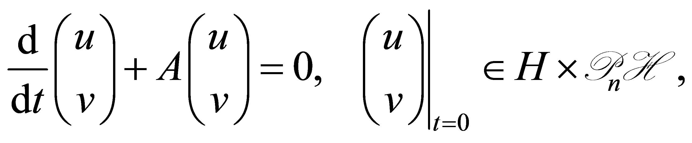
Stabilization problems for linear parabolic control systems have the history of more than three decades. Although some difficult problems are left unresolved, it seems that the study has reached a degree of maturity in a sense. The so-called dynamic compensators are introduced in the feedback loop to cope with the most difficult case such as the scheme of boundary observation/boundary input (see the literature, e.g., [1-6]). In [2-4,6], no Riesz basis is assumed, corresponding to the coefficient elliptic operators with complicated boundary operators (see (1) below). Let  be a separable Hilbert space with the inner product
  and the norm
 . A standard control system with state
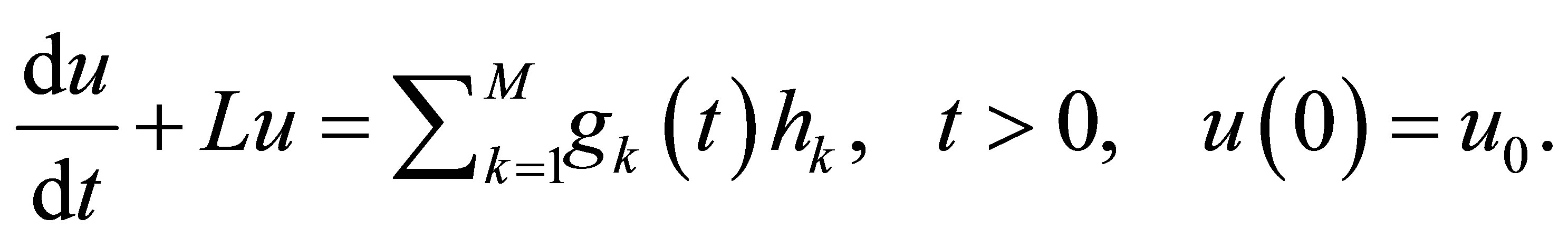
 ,
,  consists of a finite number of inputs
 ,
,  , and outputs
 ,
,  , and is described by the following linear differential equation in
 :
:
Here,  denotes a linear closed operator with dense domain
  such that the resolvent
  is compact;
  actuators through which the scalarvalued inputs
  are inserted in the equation; and
  linear functionals of
  which allow unboundedness but are subordinate to
 . The control system also reflects boundary feedback schemes by interpreting
  and the differential equation in weaker topologies. In general stabilization studies, the inputs
  are designed as a suitable feedback of the outputs
 , so that the state
  could be stabilized as
 . Then every linear functional of
  also decays at least with the same decay rate. This is true in the case where the functional is unbounded and subordinate to
 .
.
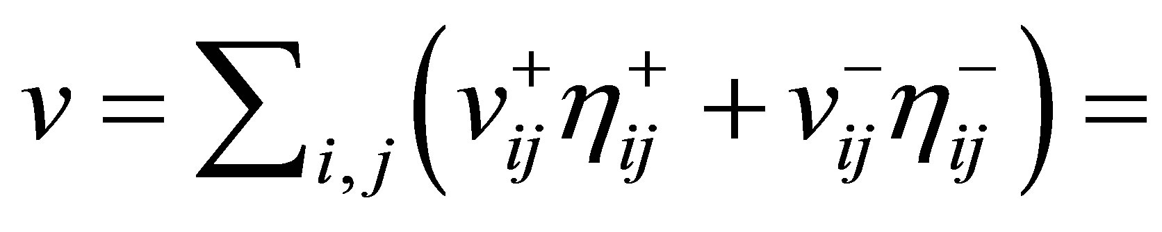
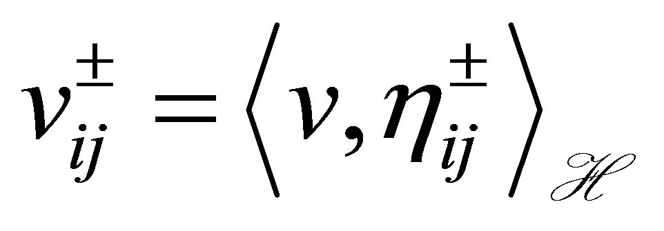
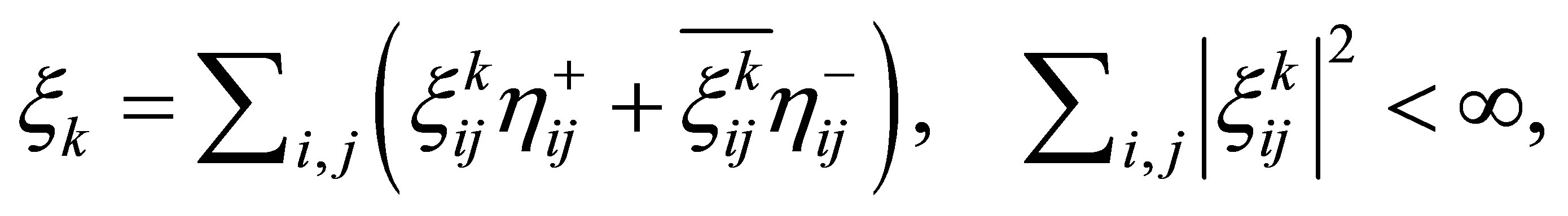
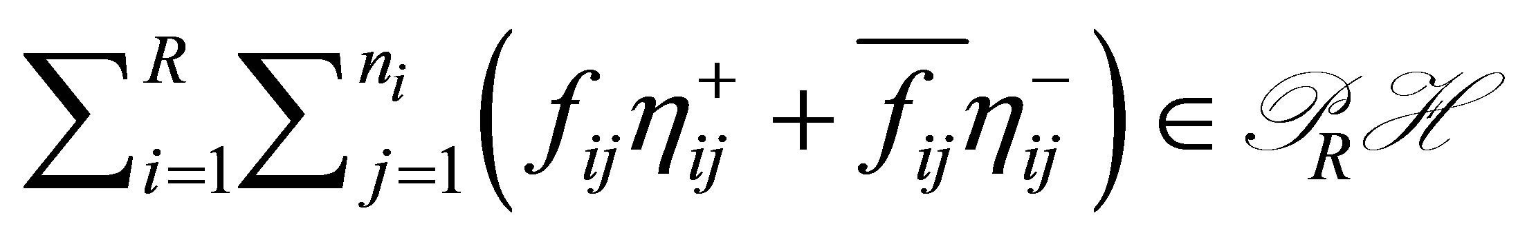
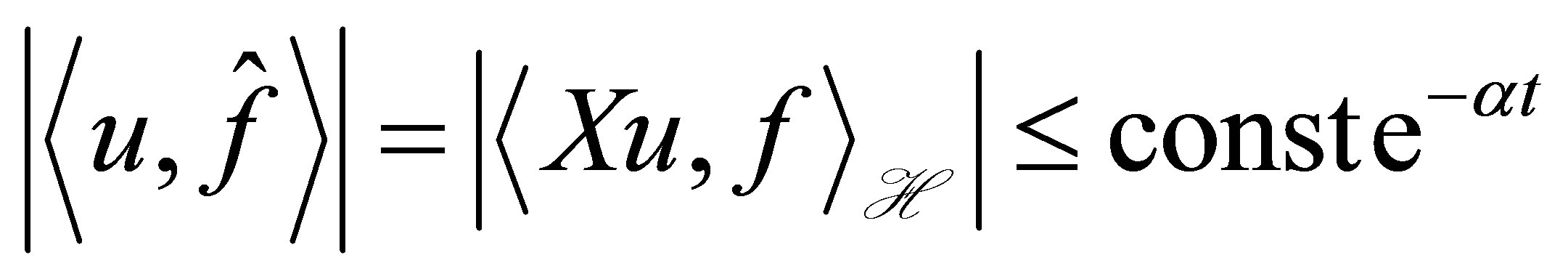
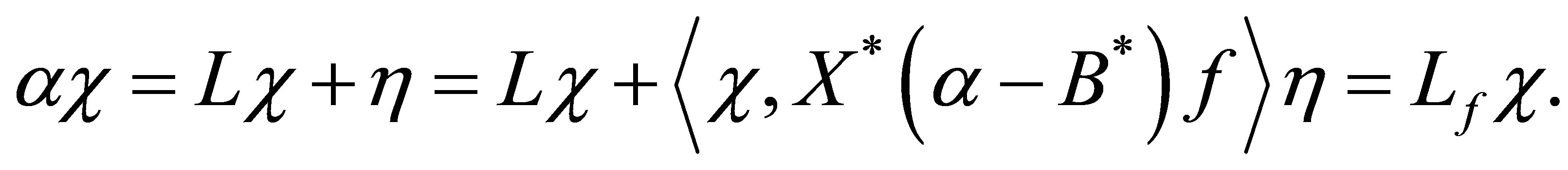
We then raise a question: can we find a nontrivial linear functional which decays faster than ? The purpose of the paper is to construct a specific feedback control system such that
  decays exponentially with the designated decay rate, and that some nontrivial linear functionals of
 , say
, say , decay definitely faster than
  for any initial state. To achieve this property, our control scheme contains a dynamic compensator with state
  in another separable Hilbert space
  in the feedback loop to connect
  and
and . Thus the control system has state
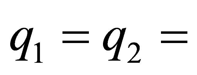
  in the product space
 . We note that the above decay property is achieved in a straightforward manner in the static feedback control scheme in which we set
  and
and ,
, . In fact, the static feedback system contains a single state
  only, and the so-called spectral decomposition of
  associated with the elliptic operator enables us to find such an
  in some spectral subspace. Such typical examples are the Fourier coefficients corresponding to higher frequencies. In our control system, however, it is indispensable in the spectral decomposition method to ensure a vector of the form
  in the spectral subspace of
  to achieve a faster decay of
 , where
  1. It is very unlikely and almost denied to find such a vector
  in our control system with state
 . To make the paper clearer and more readable, unlikeliness of the above vector
  is discussed in detail in Section 3, which turns out to be a new spectral feature of the control system, and has never appeared in the literature; this spectral property also justifies the relevance of our problem setting.
Let us begin with the characterization of the controlled plant. Let  denote a bounded domain in
  with the boundary
  which consists of a finite number of smooth components of
  -dimension. Let
  be a pair of linear operators defined by
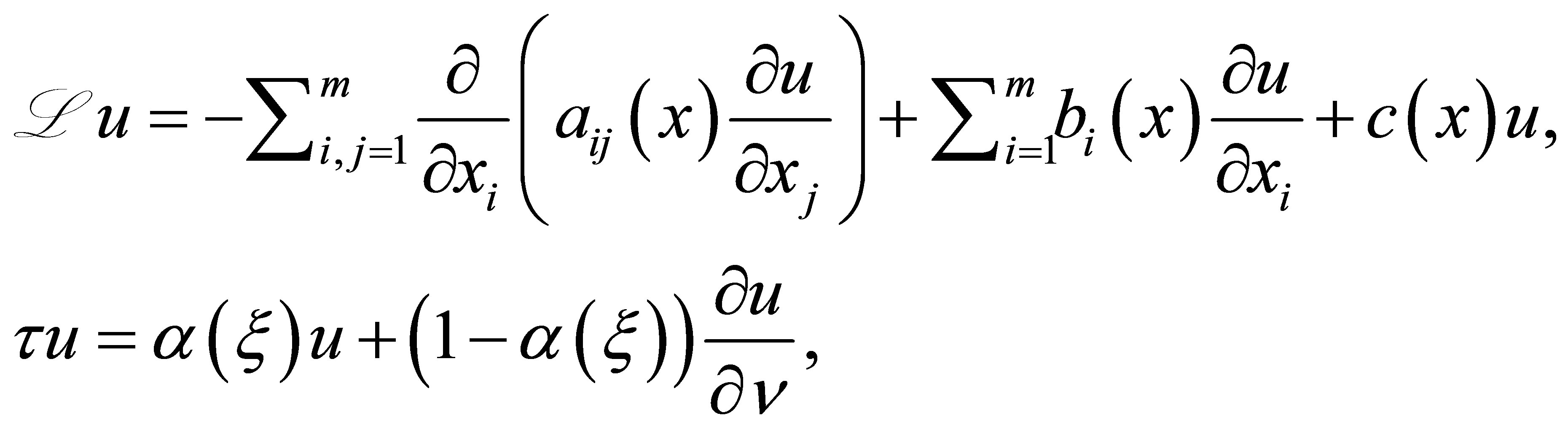 (1)
(1)
where 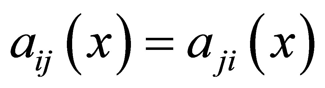 for
for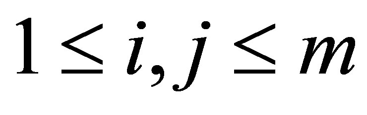 ,
, ;
;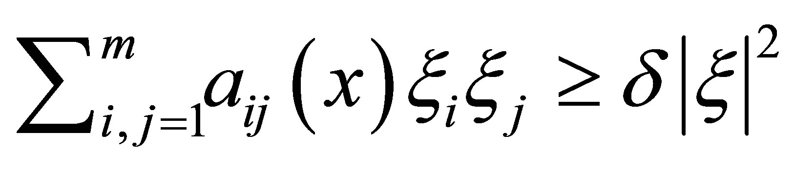 ,
,  ,
,  for some positive
  and
and
 being the unit outer normal at
 . Henceforth set
 . The pair
  defines an operator
  closable in
  as
as  for
for
 .
.
The closure of  is denoted as
 . It is well known (see [7]) that
  has a compact resolvent
 ; that the spectrum
  lies in the complement
  of some sector
 , where
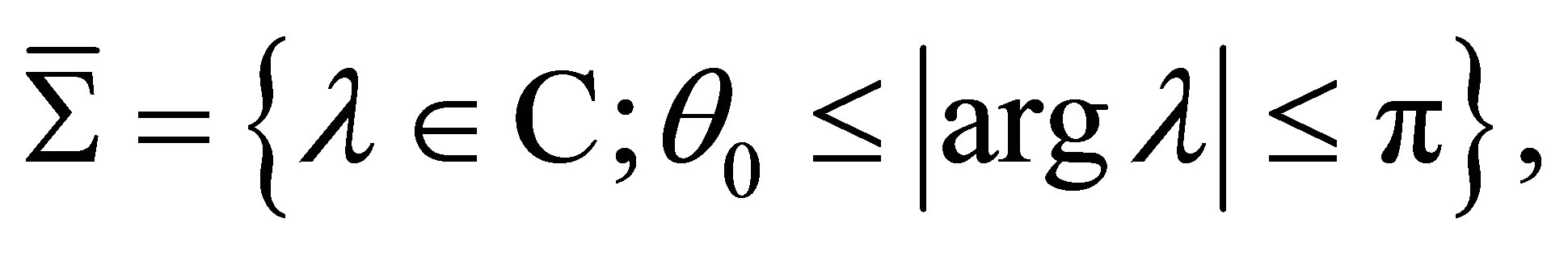
 ; and that the following estimates hold:
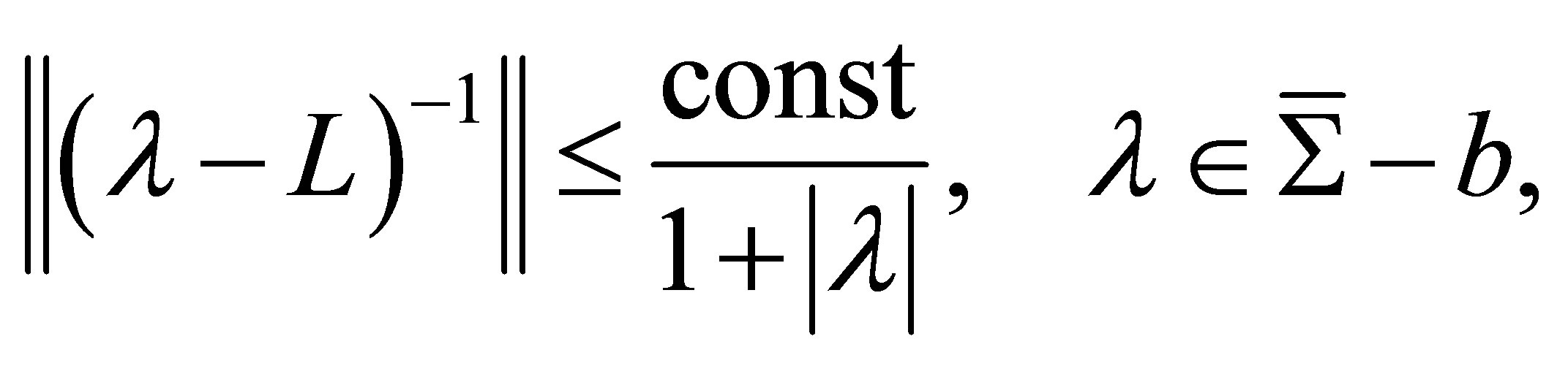 (2)
(2)
where the symbol  also denotes the
  -norm. Thus
  is an infinitesimal generator of an analytic semigroup
 ,
, . The fractional powers
 ,
,  are defined in a standard manner, where
  and
and  is sufficiently large. It is not very clear on how the domain
  is characterized by the fractional Sobolev spaces, since the Dirichlet boundary is continuously connected by the Robin boundary. Such a characterization is, however, neither essential nor necessary in our study. There is a set of generalized eigenpairs
such that
1)
;
2) for
for ; and
; and
3)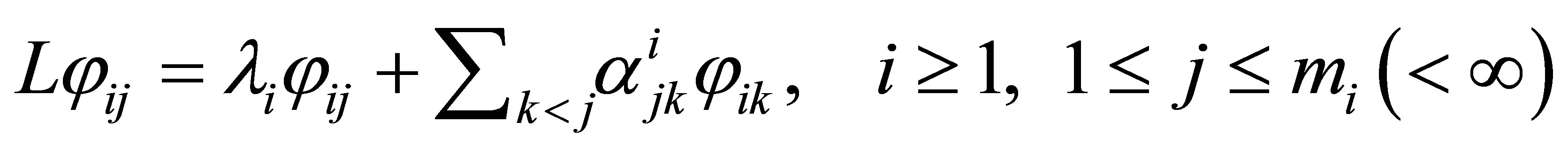 .
.
It is well known (see, e.g., page 285 of [8]) that the set  spans
spans , but does not necessarily form a Riesz basis for
 . Let
. Let  be the (not necessarily orthogonal) projector corresponding to the eigenvalue
 . The restriction of
  onto the invariant subspace
  is, according to the basis
 , equivalent to the
  upper triangular matrix
 :
:
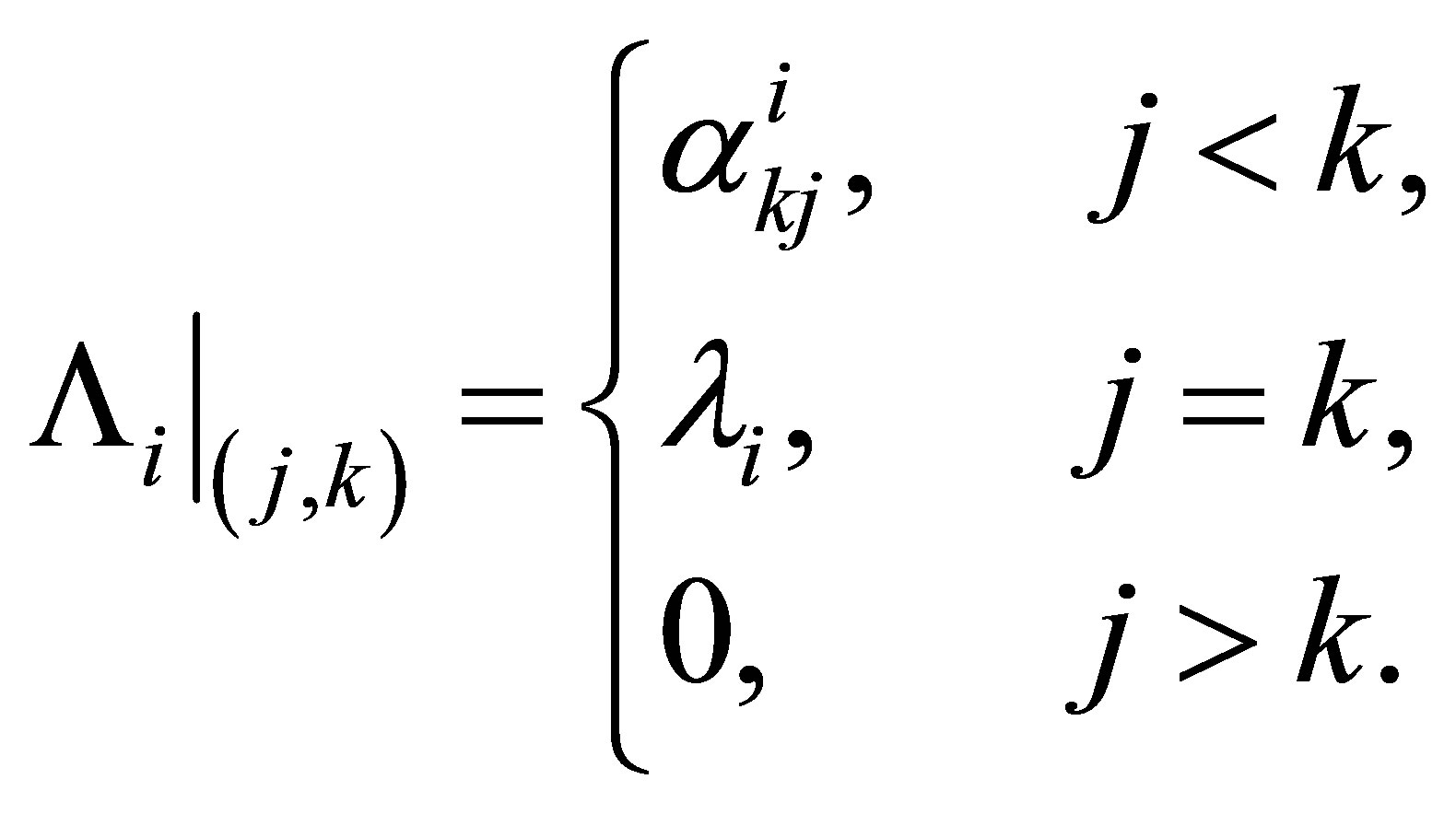 (3)
(3)
By setting , the matrix
  is nilpotent, that is,
 . The minimum integer
  such that
  is called the ascent of
 . It is well known that the ascent
  coincides with the order of the pole
  of
of  (see Theorem 5.8-A of [9] for more details). Let
  be the formal adjoint of
 :
:
 (4)
(4)
where . The pair
  defines an operator
  just as the above
 . Then the adjoint of
 , denoted by
 , is given as the closure of
  in
in . There is a set of generalized eigenpairs
such that
1) ; and
; and
2) .
.
Similarly, the set  spans
spans . Setting
 , we have the relationship:
 (5)
(5)
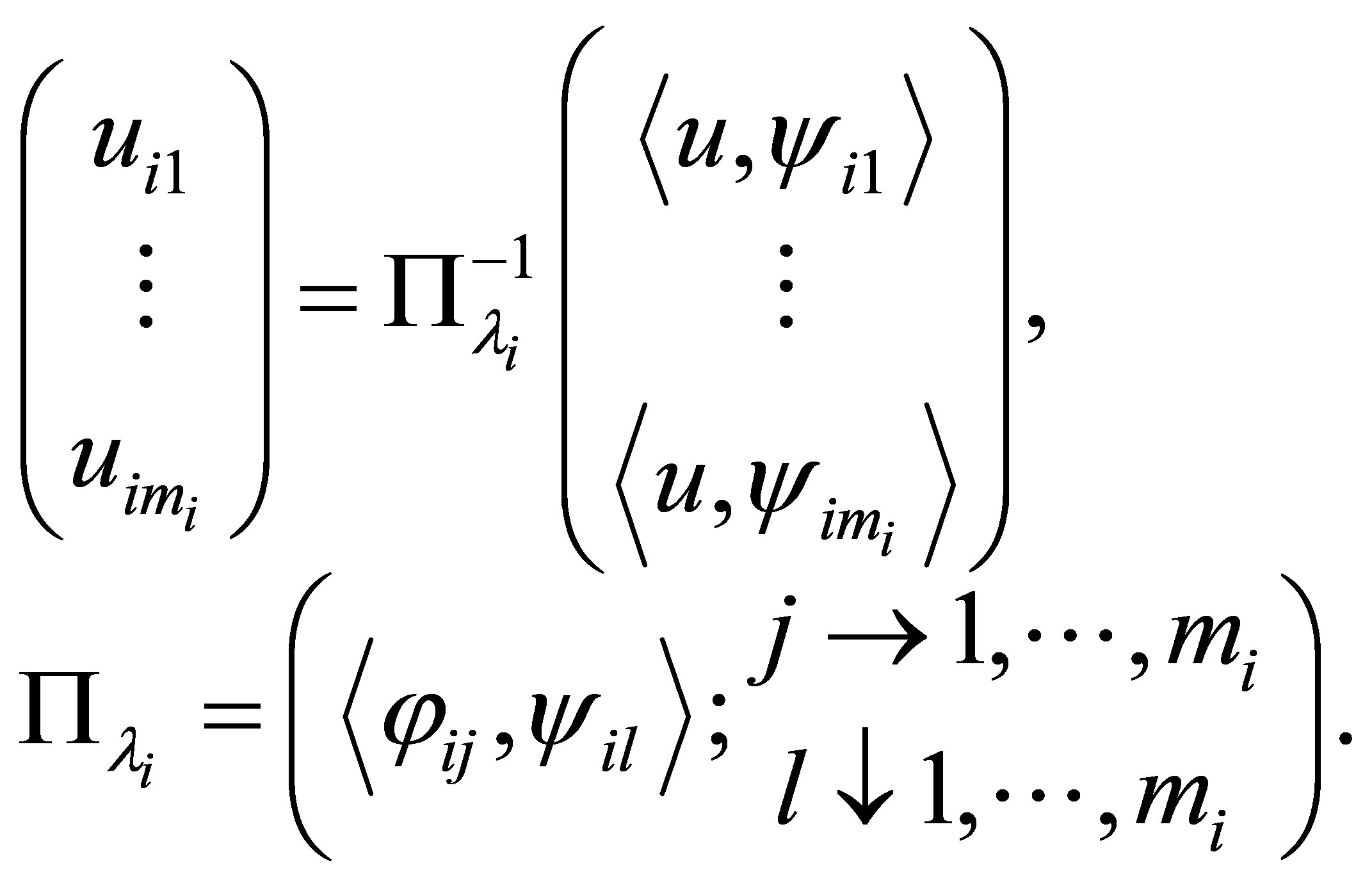
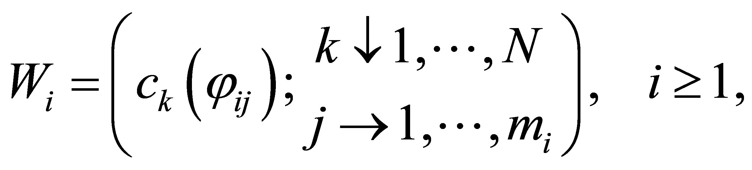
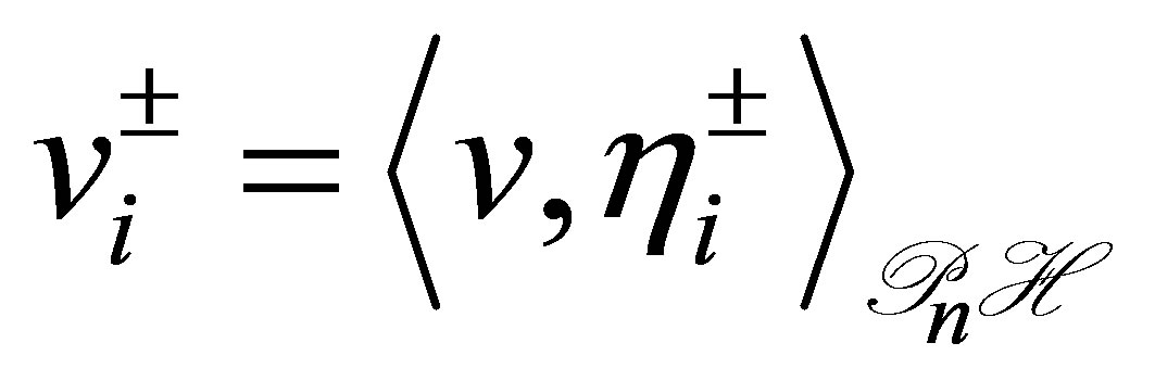
Let us turn to the characterization of a dynamic compensator. Let  be any separable Hilbert space with inner product
  and norm
 . Relabelling an orthonormal basis for
 , let
, let 
 be a new orthonomal basis for
 . Every vector
  is then expressed in terms of the basis
  as a Fourier series:
 ,
, . Let
. Let  be a sequence of increasing positive numbers:
 , and set
 , where
 . Let
. Let  be a linear closed operator defined as
 (6)
(6)
with dense domain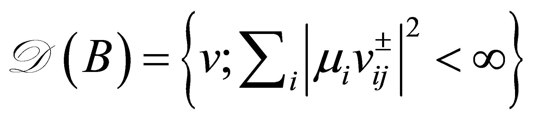 . Then, 1)
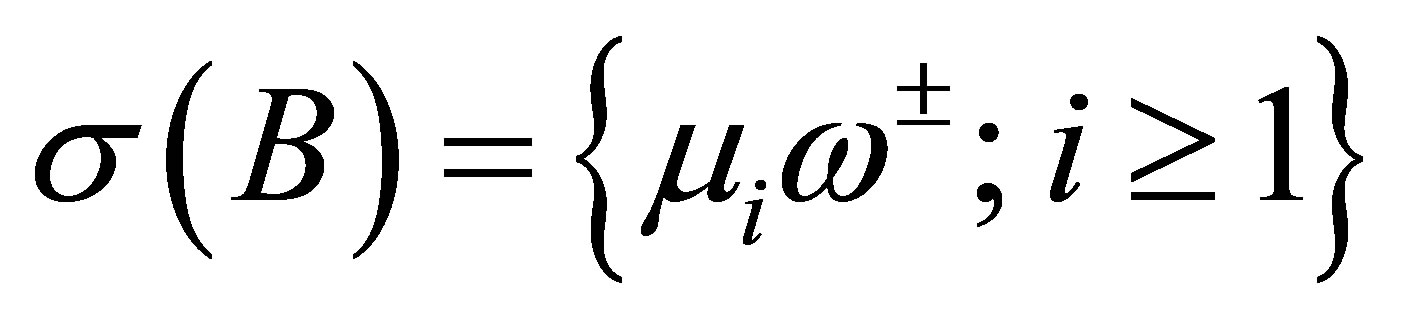 ; and 2)
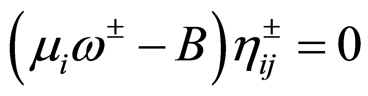 ,
,  ,
, . Thus
  is the infinitesimal generator of an analytic semigroup
 , which is expressed by
 . The semigroup
  satisfies the decay estimate
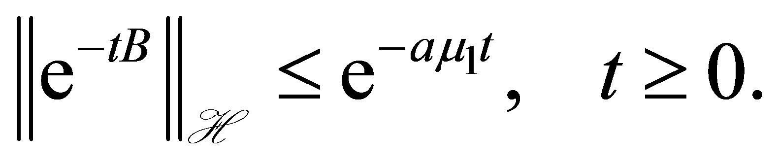 (7)
(7)
The adjoint operator  of
of  is described as
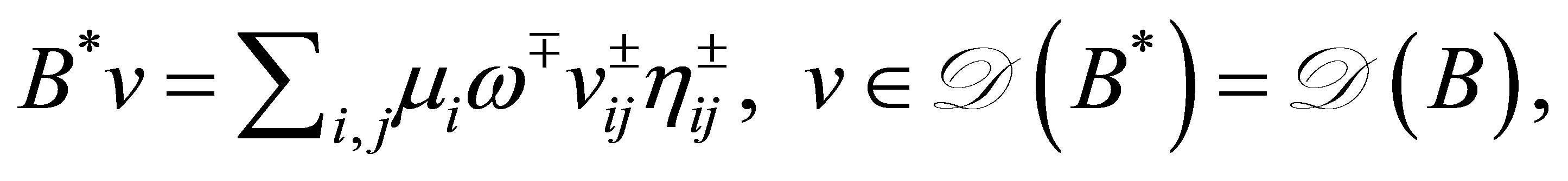 (8)
(8)
and thus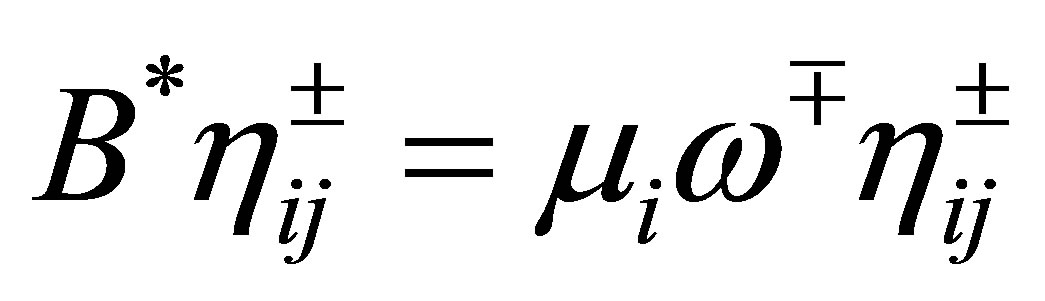 . Let
. Let ,
,  be the projector in
  such that
 .
.
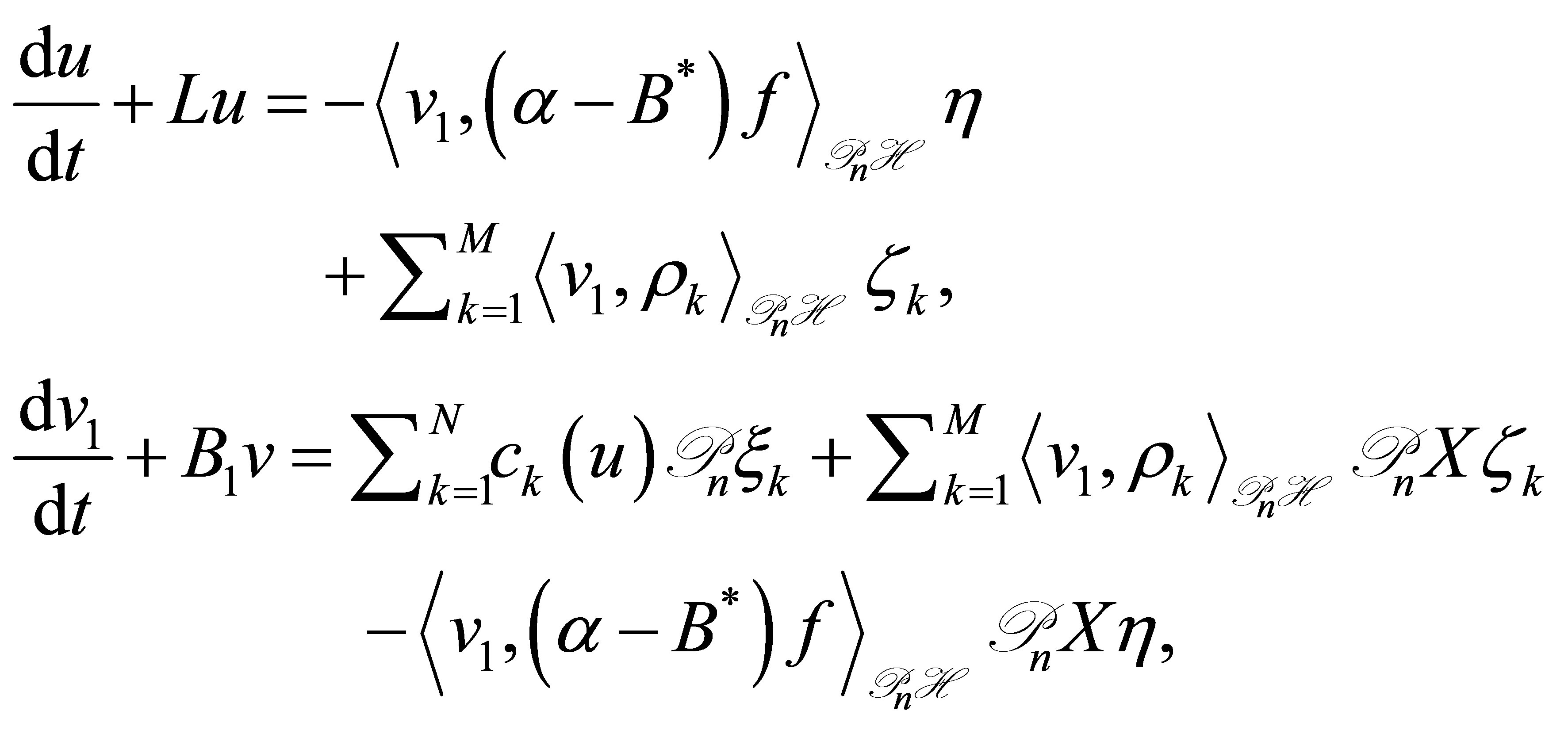
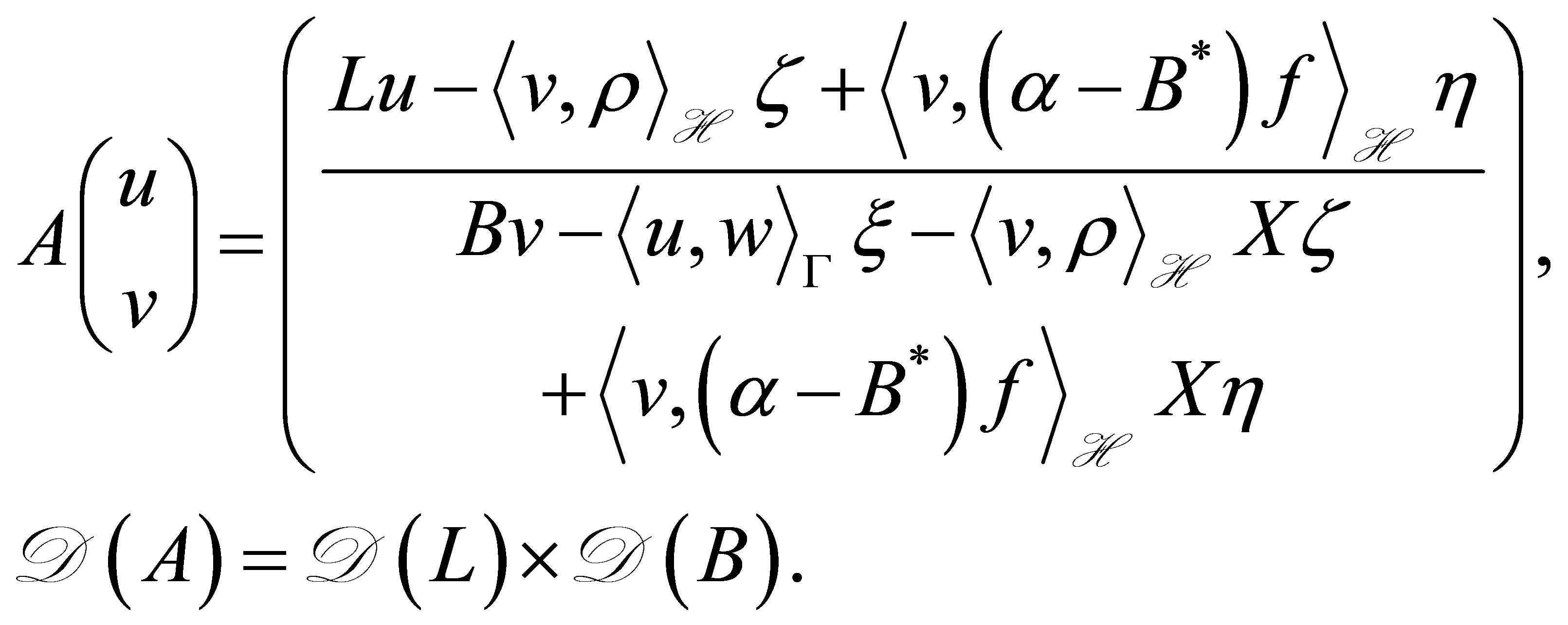
Our control system has state , and is described as a differential equation in
 :
:
 (9)
(9)
The equation with state  means a dynamic compensator equipped with a set of outputs
  and
and ,
,  , where α > 0. The parameters
  and
and  denote given actuators of the controlled plant, and
  actuators of the compensator to be designed. The outputs
  of the controlled plant are considered on the boundary, and defined as
 (10)
(10)
where  denotes observation weights. The operator
 , specified later, denotes a unique solution to the operator equation on
 ,
,
 (11)
(11)
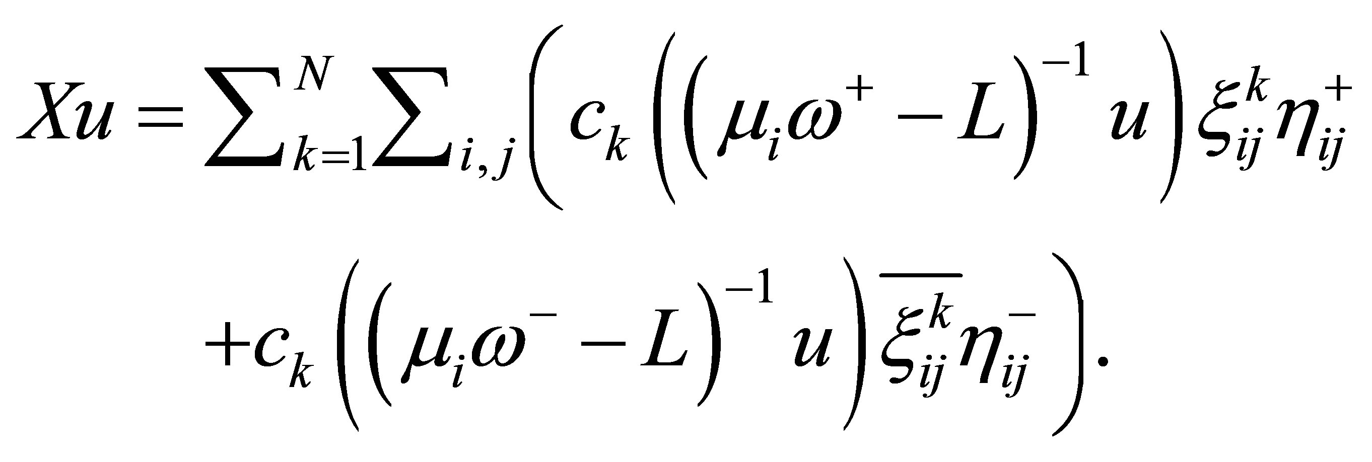
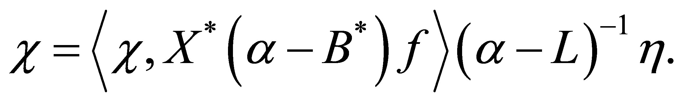
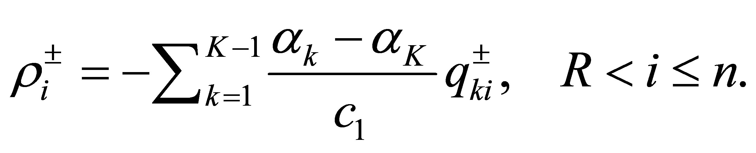
Given a suitable vector , the control law is to construct such that the number
  determines the decay rate of a functional
 , where
 . As we see later, the roles of the outputs
  and
and  are, respectively, to determine the decay of
  and the decay of
 . In state stabilization problems only, the output
 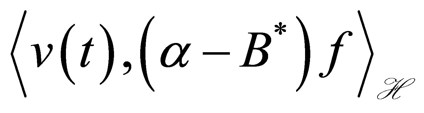 does not appear. More precisely, let
  be a number such that
 . We seek a new feedback scheme such that the decay estimates
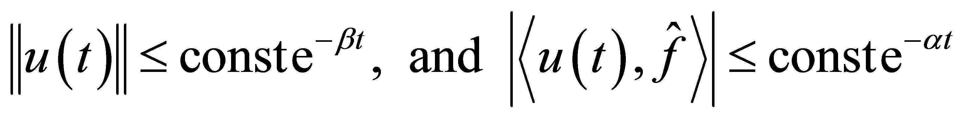 (12)
(12)
hold for every initial value and , such that the decay of
  is no longer improved. To achieve the non-standard decay (12), introduce a new operator
 (13)
(13)
and assume conditions in terms of . These conditions have never appeared in the literature. Note that conditions are posed on
  for state stabilization.
The functional  may be regarded as a kind of output of the system. It is worthwhile to refer to our previous results on output stabilization [10-13]: In [10], the decay of outputs is discussed with lack of observability conditions, but the relationship of the decay between
  and the outputs is unclear. In [11-13], the problem is discussed, based on a different principle, i.e., a finitedimensional pole assignment theory with constraint. The controlled plants are, however, limited to those equipped with Riesz basis, and the actuators of the controlled plant, corresponding to our
 , are restrictive, and must be subject to a strong constraint: the actuators have to be designed so that their spectral elements in each spectral subspace are orthogonal to the weights of the outputs at infinity. As we have seen, the controlled plants in the present paper do not necessarily allow a Riesz basis, although a somewhat stronger condition, i.e., complete observability, is assumed. An example of systems equipped with complete observability is illustrated in the end of Section 2.
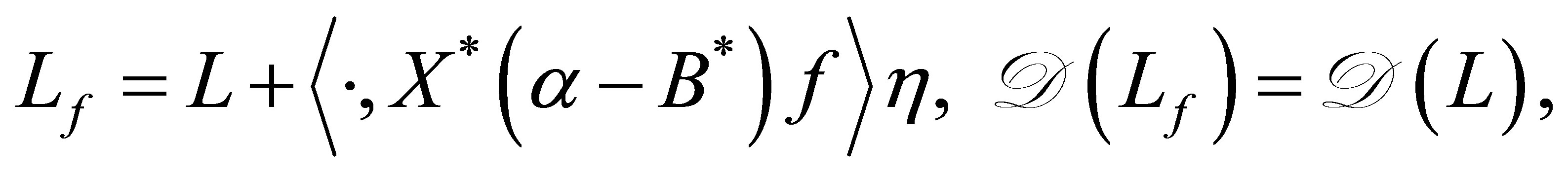
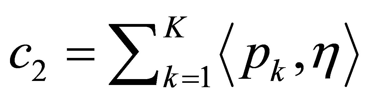
The feedback law in (9) contains parameters: ,
,  ,
,  ,
,  ,
,  ,
,  , and
, and  to achieve the nonstandard decays (12). They are designed in the following manner: 1) The actuator
  is given in advance arbitrarily. 2) Given the parameters
  and
and , the operator solution
  is ensured. 3) Then, a vector
  is chosen among a very wide range of sets in
 . 4) Finally,
  , as well as
 , are designed to satisfy a finite number of controllability conditions associated with the new operator
 . It is generally desirable to pose less restrictive assumptions on the actuators of the controlled plant. In fact,
  is arbitrary, and, as we see later that the conditions on
  are much less restrictive than those in our preceding works above. In fact,
  only have to be designed, belonging to an infinite dimensional subspace of
 .
.
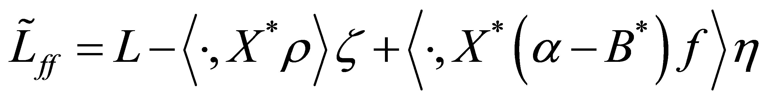
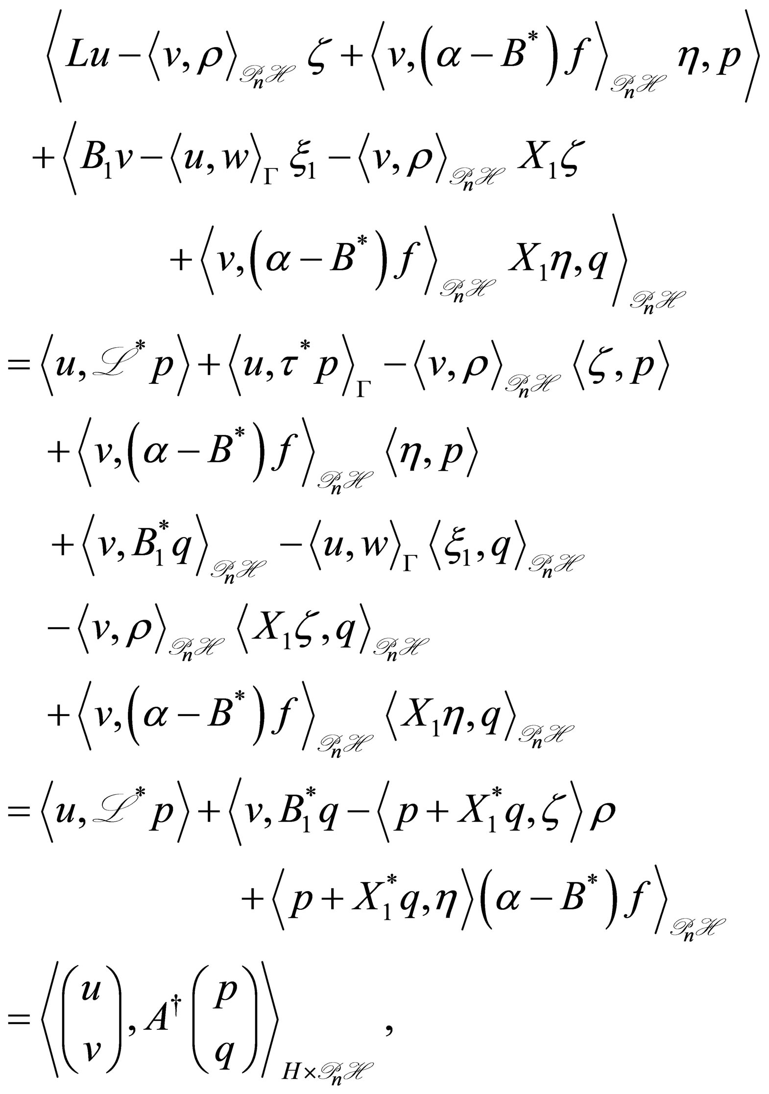
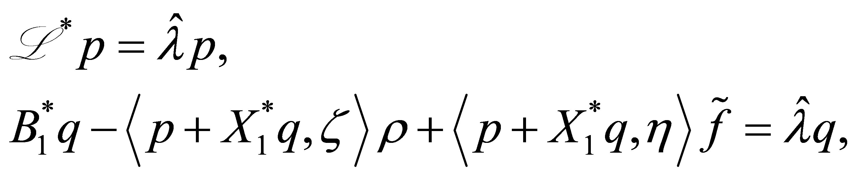
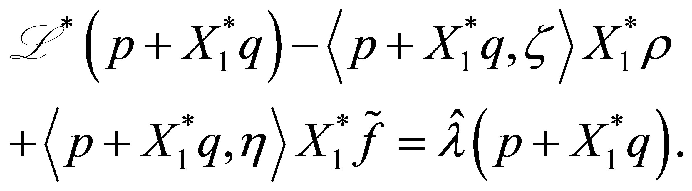
Our main results consist of Theorem 4 in Section 2 and a series of assertions in Section 3 (Theorem 7, Propositions 8, and Theorem 9): The former is on the control law ensuring the non-standard decays (12), and the latter on the relevance of the problem setting with Equation (8), which discusses a spectral property of the invariant subspaces in  associated with the coefficient operator in (9), that is, unlikeliness of a vector of the form,
  in these subspaces. In Section 3, the spectrum of the coefficient operator is characterized (Theorem 9). To the best of the author’s knowledge, the latter has never been discussed so far, and clarifies a new property of internal structures of control systems.
2. Decay Estimates of Solutions
To ensure well-posedness of our control system (8), let us begin with the operator Equation (10). Adjusting  and
and ,
,  , we may assume that
 (14)
(14)
(see (2) for ). In (9), let us express the actuators
 ,
,  as Fourier series in terms of
 :
:
where the overline denotes the complex conjugate. Before stating our first result, let us define the matrices , and
, and ,
,  by
by
 (15)
(15)
and
 (16)
(16)
respectively. Then our first result is stated as follows:
Theorem 1. 1) By assuming (14), the operator equation (11) on  admits a unique operator solution
 , which is expressed as
 (17)
(17)
2) Assume further that
 (18)
(18)
Then we have . Here,
  denotes the closure of
  in
in .
.
Remark. 1) The first condition in (18), called the complete observability condition, is fulfilled with  in the case where
 ,
,  ,
, . Actually, by choosing the
  with
with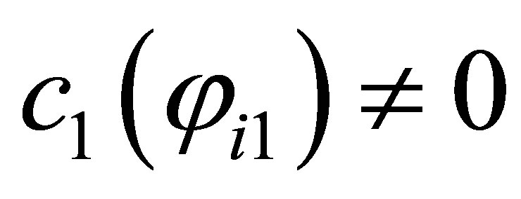 ,
,  , the condition is fulfilled. In the case where
 ,
,  , however, the condition means that
 ,
,  , which requires that
  be equal to or greater than
 : this is the case, for example, where
  is selfadjoint.
2) The condition:  is the so called finite multiplicity condition. In the case of
 , we know that
 ,
, . Thus, by choosing
 , the complete observability condition is automatically fulfilled. As another example, let
  be a self-adjoint operator defined by
  in
in  equipped with the Dirichlet boundary. The eigenvalues of
  consist of
 ,
,  ,
,  , where
  are the zeros of the Bessel functions
  of m-th order. It is expected that
 , if the well known Bourget’s hypothesis (see pp. 484-485 of [14]) is proven. As long as the author knows, this conjecture has not been proven so far.
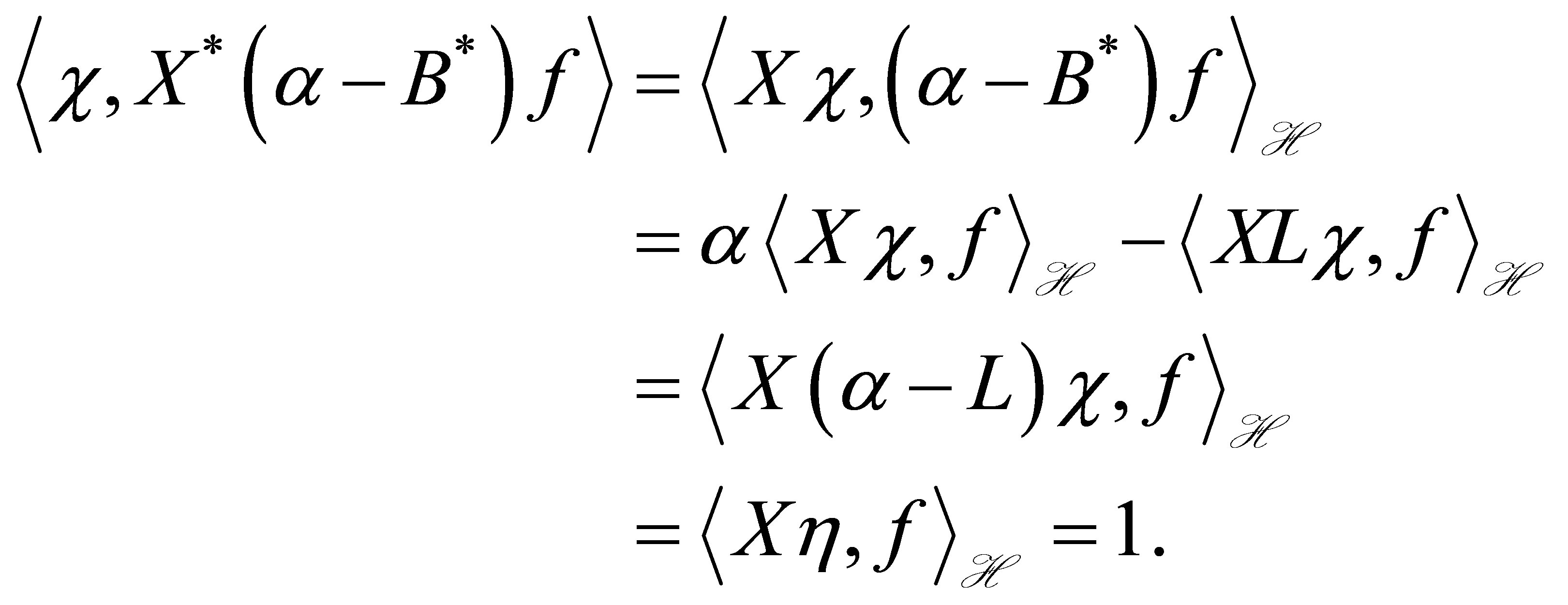
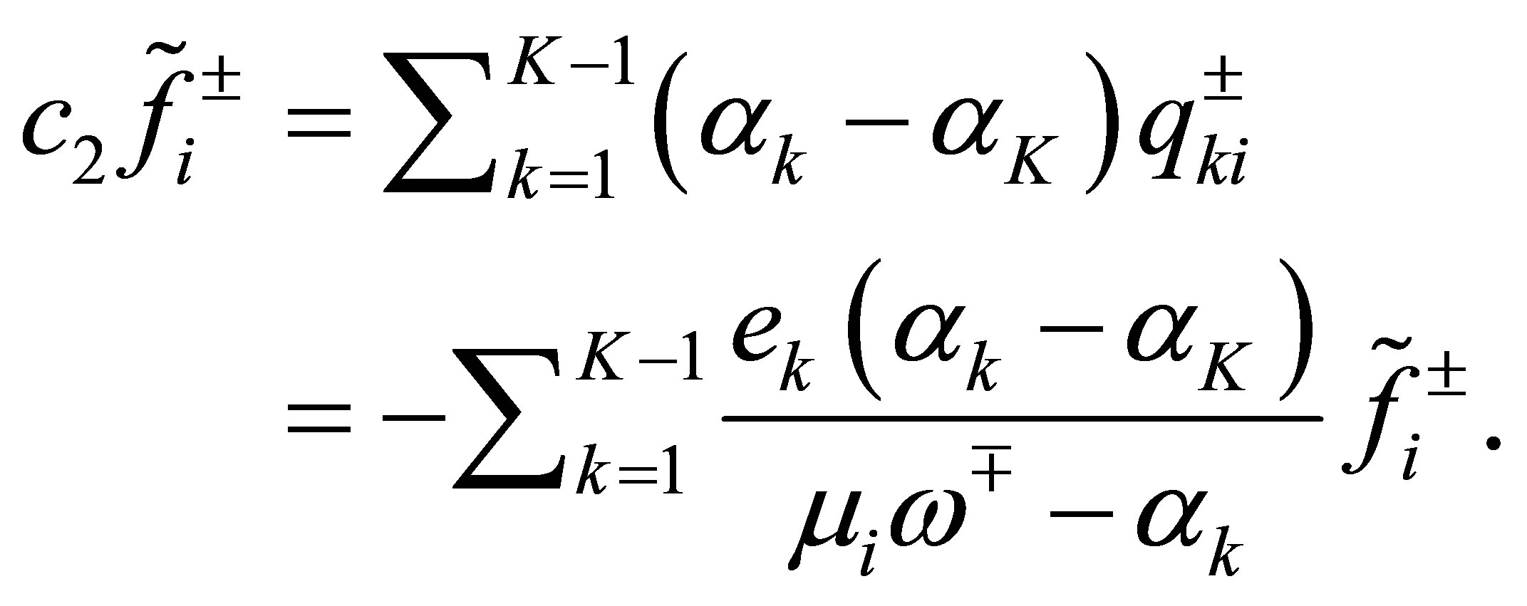
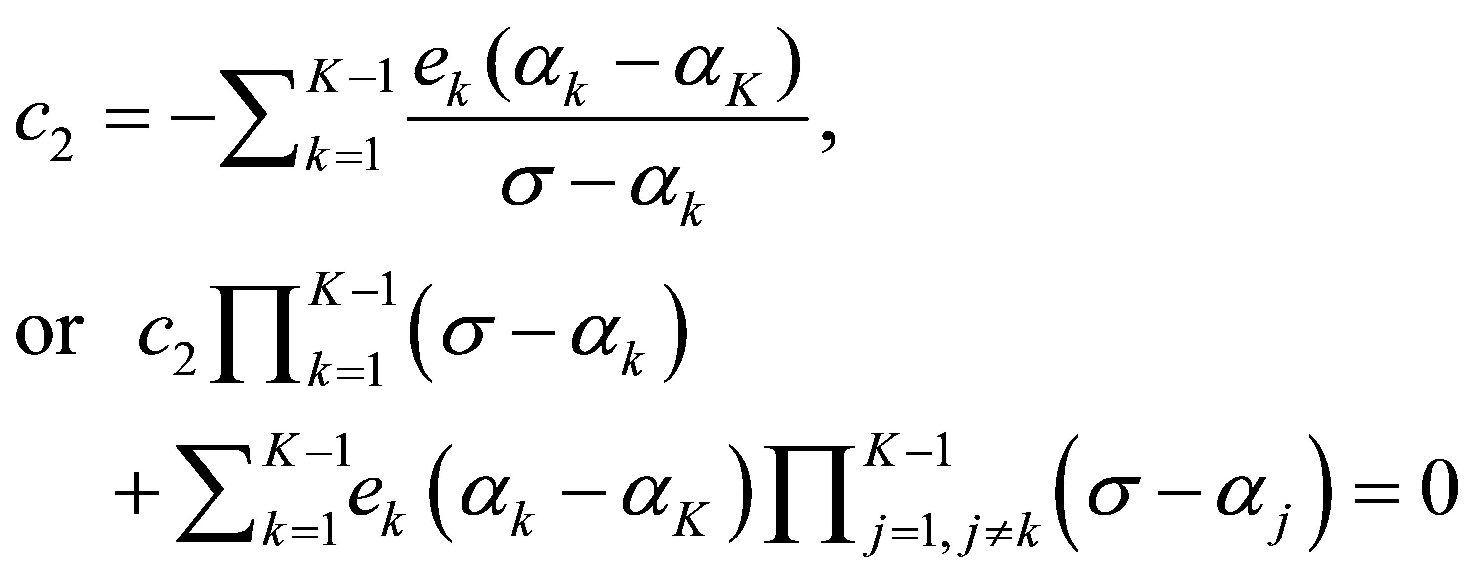
Proof. The result is a version of the results in [2-5], so that we give here only an outline of the proof. 1) Expression (17) and uniqueness of  are examined in a straightforward manner.
2) Relation  is equivalent to
 . Assuming that
 , we see by (17) that
Since , we see that
  for
for  and
and .
.
For a  such that
  and each
 , we introduce a series of meromorphic functions
 ,
,  by the recursion formula:
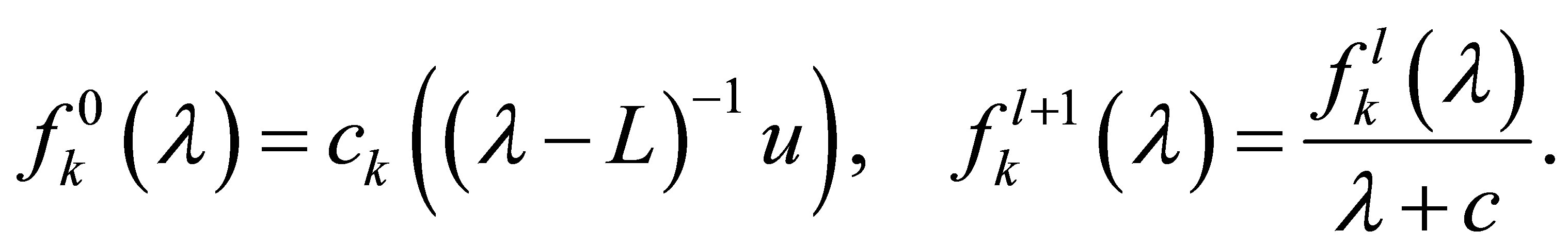 (19)
(19)
Each function  has the properties: 1) It has at least the zeros
 ,
, ; and 2) the algebraic growth rate
  of these zeros,
  is smaller than 2 by (14). These properties combined with Carleman’s theorem [15,16] imply that
  for
for ,
,  ,
, . Following [5], we calculate the residue at each
 . Then, we see that
 (20)
(20)
Let . Note that the restriction of
  on
on  is equivalent to the matrix
 , and thus,
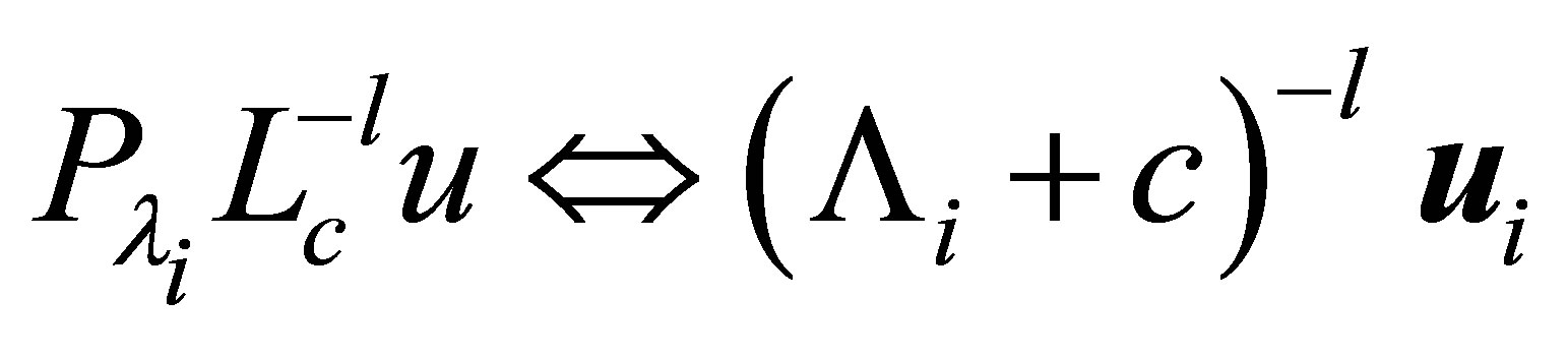 . The relation (20) is rewritten as
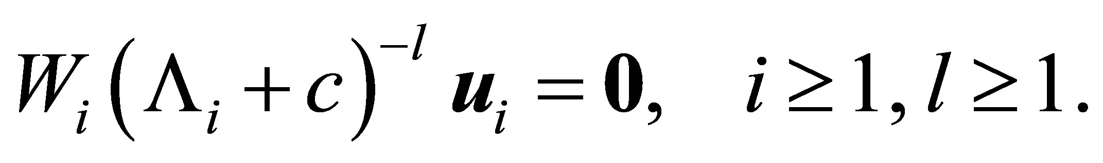 (21)
(21)
The complete observability in (18) implies that 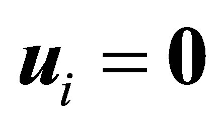 for
for . In view of (5), we see that
  for every
  and
and . Since the set
  spans the whole space
 , we conclude that
 . Q.E.D.
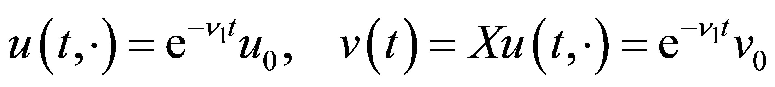
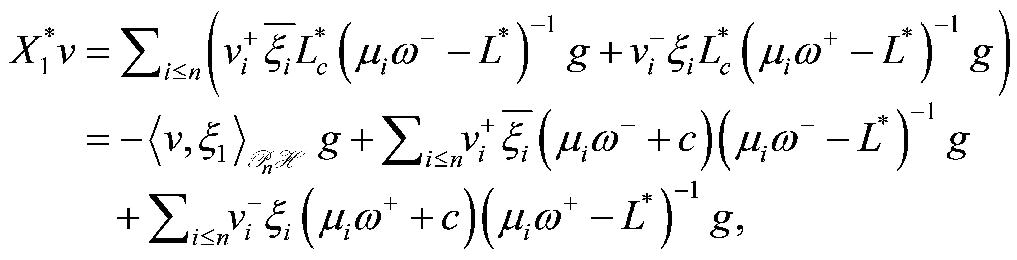
Decay of solutions to Equation (9): In view of (11), it is easily seen that ,
,  , or
, or . Thus,
 (22)
(22)
for . In (9). let
 , and
, and  (see Proposition 2). Equation (9) contains various parameters:
 ,
,  ,
,  ,
,  ,
,  ,
,  , and
, and , among which
 ,
,  and
and  are already determined in Theorem 1. Let a non-trivial
  be given arbitrarily. Then,
  by Theorem 1. We find a non-trivial vector
 such that
 (23)
(23)
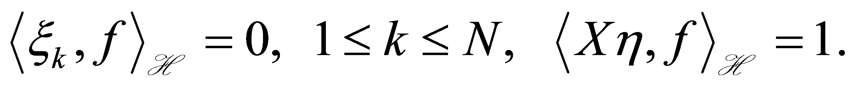
There is a variety of choice of such an . In fact, this is simply possible, e.g., by finding
  such that
for . Then
  does not belong to the space spanned by
 ,
, . The integer
  may be chosen arbitrarily large. The vectors
  will be determined in terms of the operator
 .
.
The state  in (9) satisfies the equation:
Actuators  are chosen so that
 ,
, . An assumption on these
  will be discussed later (see (28)). Then, it is immediately seen that
 (24)
(24)
By the decay (22), we obtain the estimate:
 (25)
(25)
for . Here,
 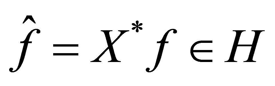 is non-trivial.
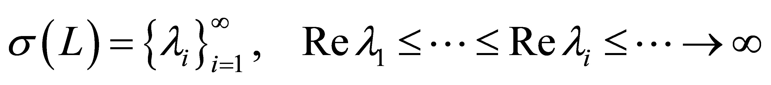
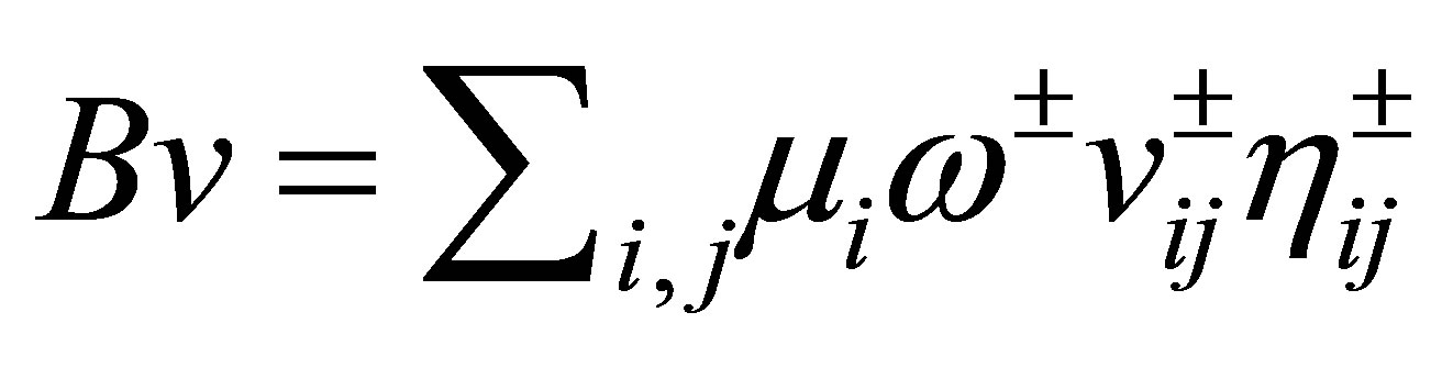
The operator 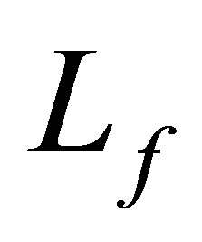 defined in (13) has a compact resolvent, and
  consists only of eigenvalues. Let
 (26)
(26)
where  and
and  for i ≠ j. Each
  may admit generalized eigenfunctions. Let
  be the projector corresponding to the eigenvalue
 which is calculated as
 , Ci
, Ci
being the small counterclockwise circle with center . Then
Proposition 2. 1) The number  belongs to
 . 2) Any generalized eigenfunction of
  in
in 
 and
and  are orthogonal to each other.
Proof. 1) Suppose that there is a  such that
 . Then,
 . Thus we have, as a necessary condition,
Now set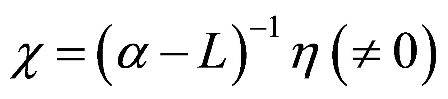 , and calculate as
Thus we see that
2) Let ,
,  , and
, and  ,
,  , possible generalized eigenspaces of
 . For a
 , we calculate by (23) as
This implies that , or
, or . Suppose then that
 ,
, . For a
 , the function
  is in
is in , and
, and  . The same calculation as above immediately shows that
 . Thus,
 (27)
(27)
The integer  varies over a finite set of positive integers depending on
 . Q.E.D.
We now choose the actuators  in (9) such that
 (28)
(28)
Then,  by the above proposition. All parameters except for
  in (9) are determined.
Rewrite the equation for  in (9) as
 (29)
(29)
Let us introduce an operator  as
as
Let the integer  be such that
 . Then,
  ,
, . The following proposition is just a simple version of the result in [17].
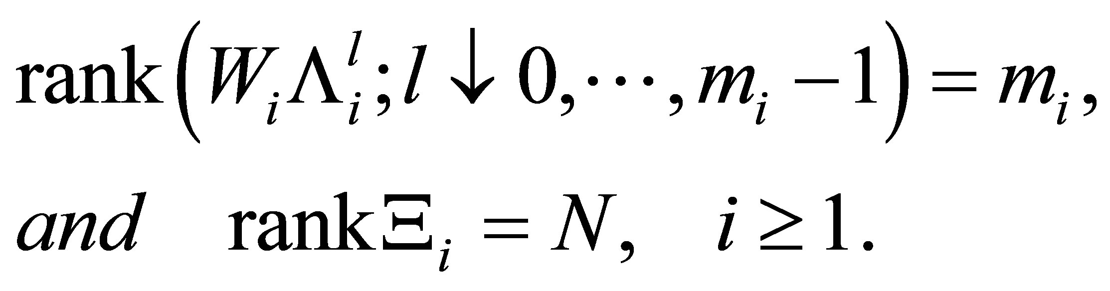
Proposition 3. Let  be the projector defined by
 . Choose a
  such that
 . Suppose that the pair
  is a controllable one. Then we find
  such that
Thus, 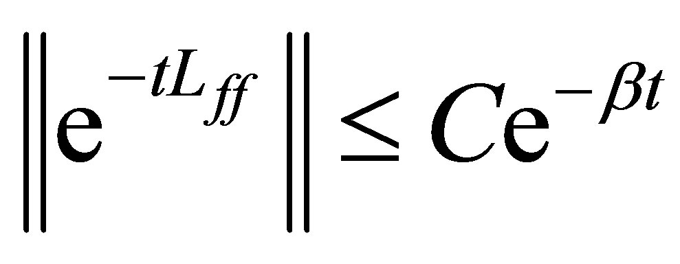 ,
, . We are ready to state the non-standard deay of solutions to Equation (9).
Theorem 4. Let  such that
 . Suppose that
1) and
and  satisfy the rank conditions (18);
2)  is arbitrarily given;
3)  is chosen to satisfy (23); and 4)
  satisfiy the controllability condition in Proposition 3.
Then we find a large integer ; vectors
 ; and a postive
  close to
 , and subsequently the control system in the product space
 ;
;
 (30)
(30)
where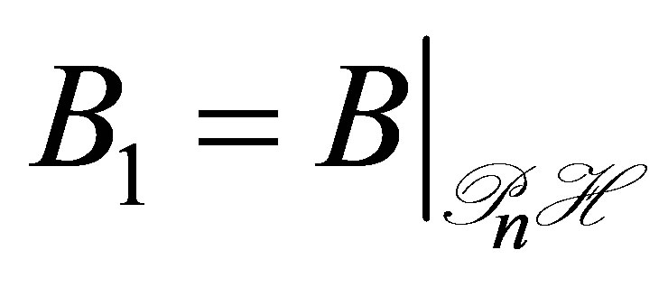 . Every solution
 satisfies the decay estimate:
 (31)
(31)
for . The estimates for
 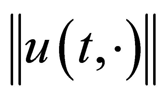 and
and 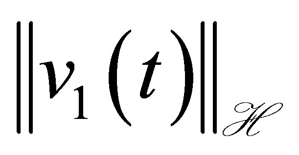 can be no longer improved.
Proof. Choose the functions ,
,  stated in Proposition 3. In view of Theorem 1, we find
  such that
  arbitrarily approximate
  in the topology of
 . Since
  is separable, we may assume with no loss of generality that these
  are constructed in
  for an enough large
 .
.
Let us consider the operator  and the perturbed
 . The right-hand side of (29) is dominated by the decay estimate (22). Since
  are chosen close to
 , the semigroup
  is stable, and satisfies the standard estimate:
 (32)
(32)
where . Thus every solution
  to Equation (9) satisfies the estimate:
 (33)
(33)
where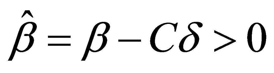 . The decay estimate for the functional
  is already obtained in (25).
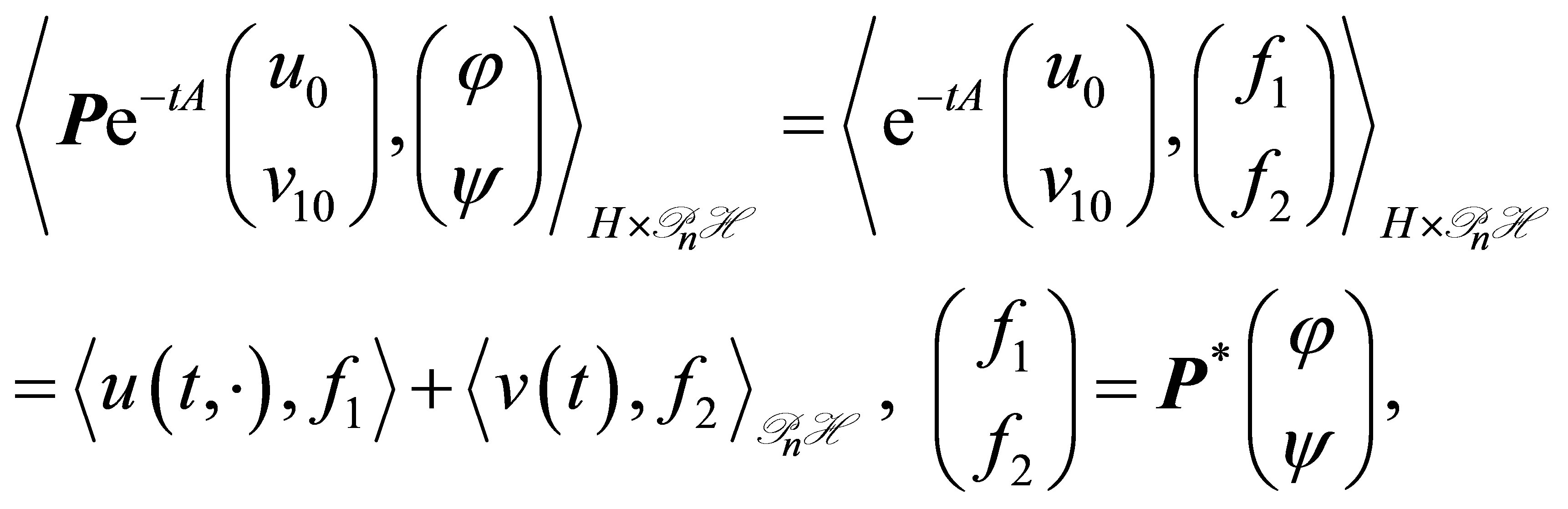
The control system (30) is derived in the following manner: Set , and apply the projector
  to the equation for
  in (9). By noting that
 , then, (30) is immediately obtained. Equation (30) is clearly well posed in
 : Thus every solution to (30) is derived from the solution
  to (9) with initial value
  such that
 , by setting
 . Thus the first estimate of (31) is derived from (33). The second estimate of (31) is clear by (25).
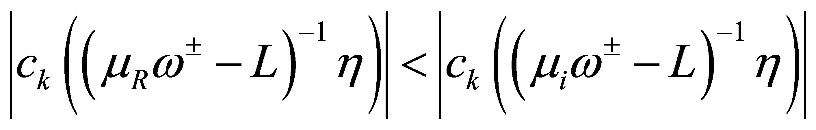
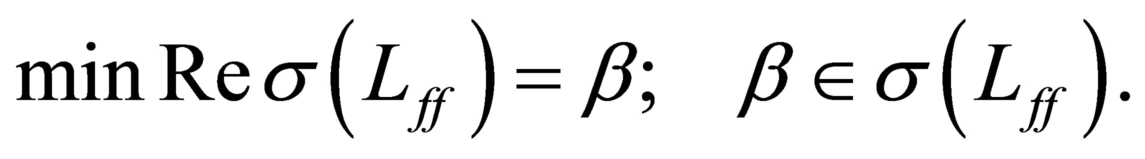
Finally we show that the first estimate of (31) for  is no more improved. The spectrum
  of the perturbed operator
  consists only of eigenvalues. It is expected that the value of
  would be close to
  as long as
  are close to
 : When both
  and
and  are selfadjoint, it is well known—via the min-max principle (see [18])—that each eigenvalue of
  is continuous relative to the coefficient parameters. In our problem, the following result holds:
Proposition 5. The minimum of  is continuous relative to
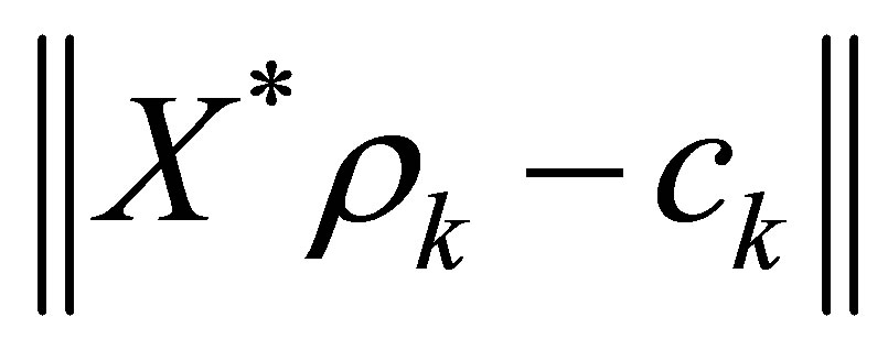 ,
, .
.
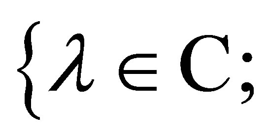
Proof. Set
 . In view of (32), the left half-plane:
  is contained in
 . Thus we see that
 . Choose an
  enough small so that
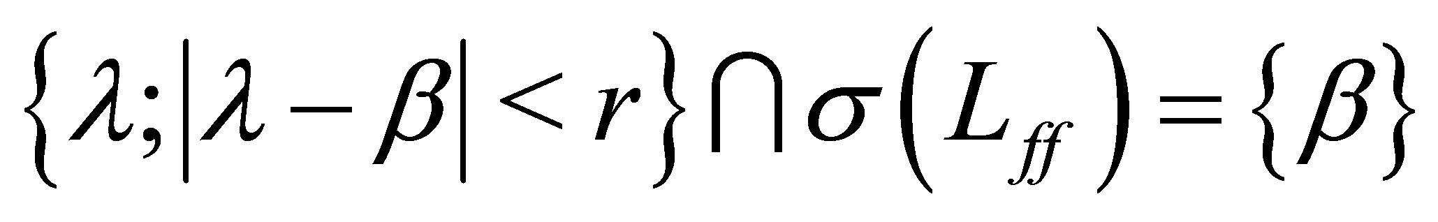 . Let
. Let  be the counterclockwise circle:
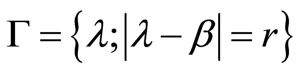 , and suppose that
 for
for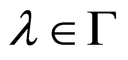 . Choose
  such that
 . Then,
  belongs to
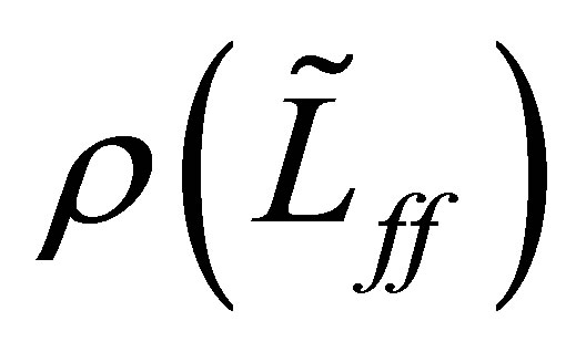 . In fact, we have the relation:
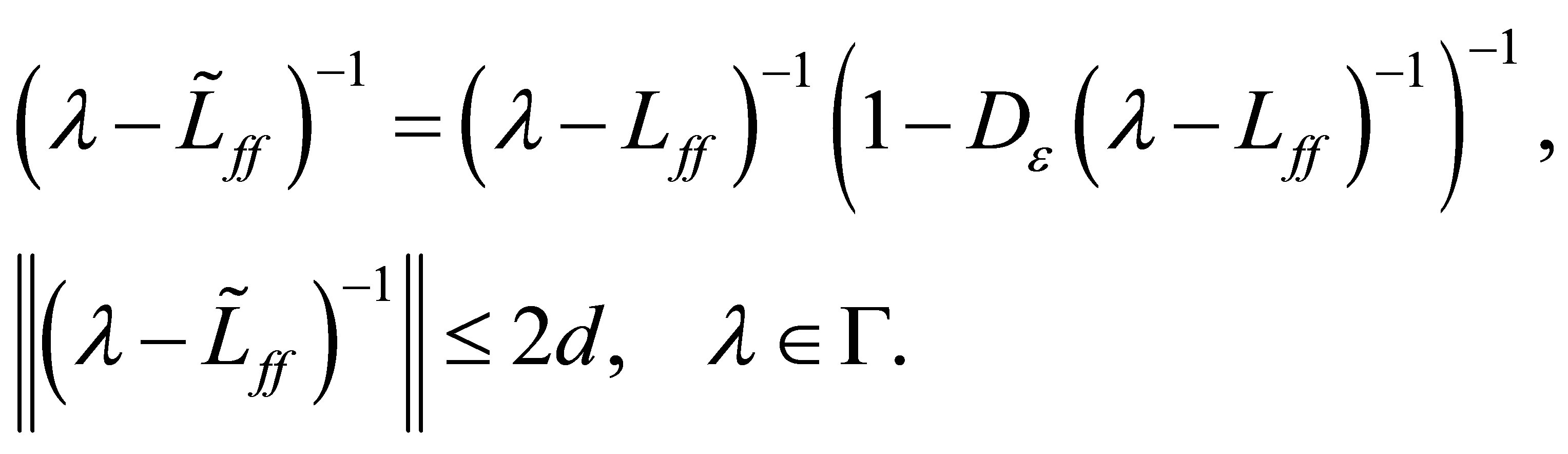 (34)
(34)
Recall that, for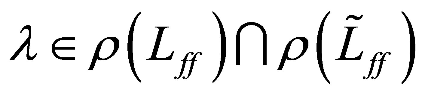 , the (second) resolvent equation:
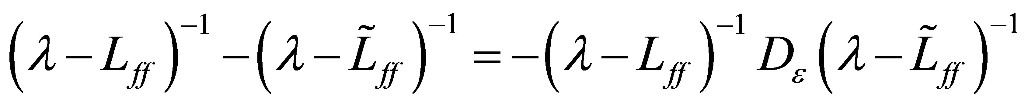
holds. Then we see that
 (35)
(35)
The first term of the above left-hand side of (35) is the projector, corresponding to the eigenvalue  of
of . Choose
  closer to
 , if necessary, so that
Supposing that  is contained in the half-plane:
 , we then derive a contradiction. If so, the resolvent
  is analytic inside and on
 . Thus the second term of the left-hand side of (35) must be equal to 0. Let
  be an eigenfunction of
 , corresponding to the eigenvalue
 . Then,
The right-hand side is, however, estimated as follows:
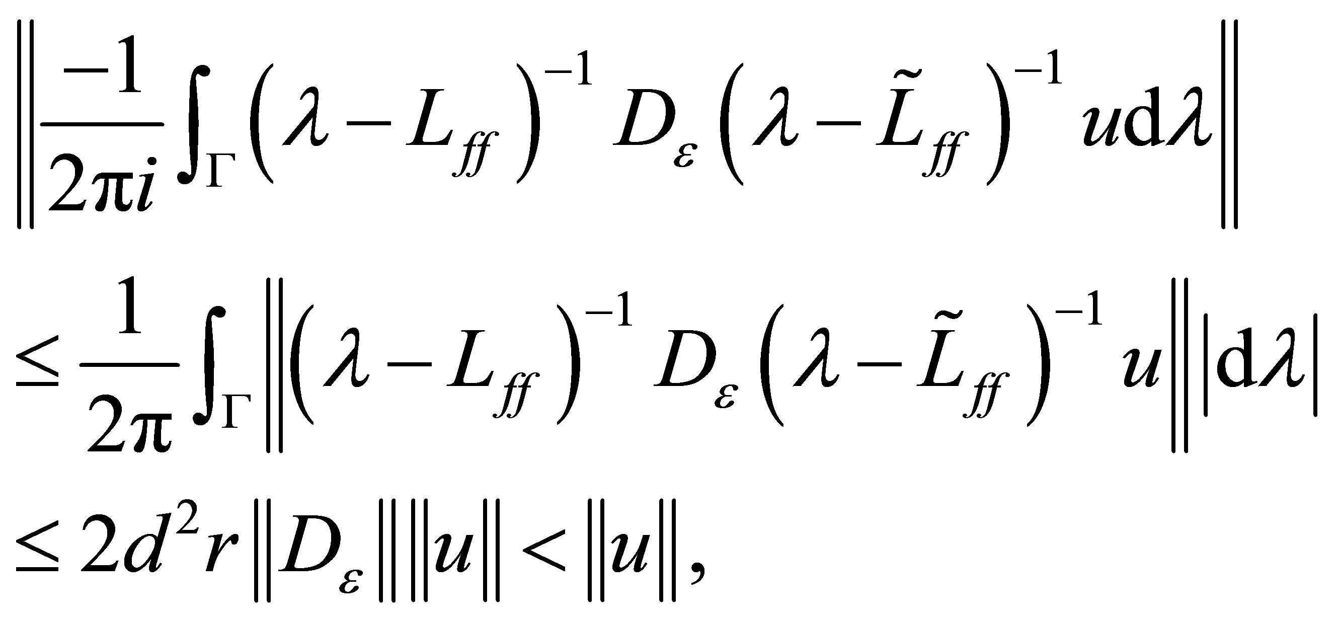
which is a contradiction. Therefore, the spectrum  also lies in the left-half plane:
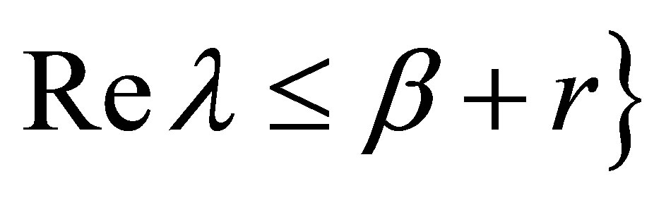
 . As a conclusion, the minimum of
 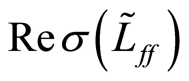 satisfies the estimate:
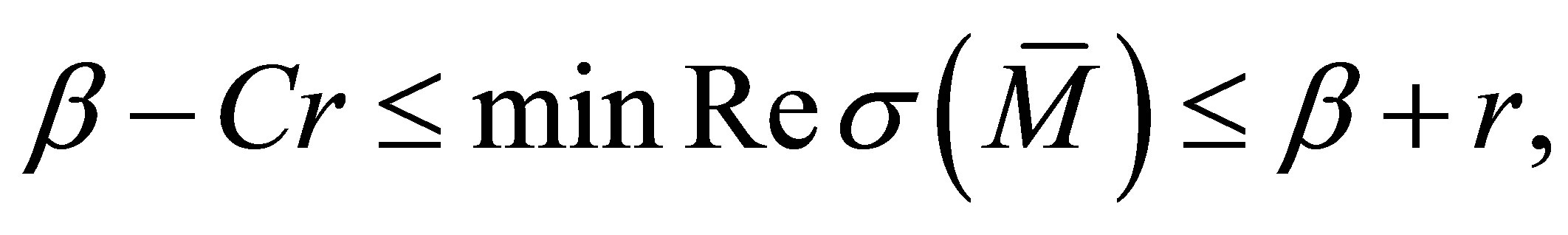
as long as ,
,  are small. Q.E.D.
Let us turn to the proof of Theorem 4. Choose an  in Proposition 5 such that
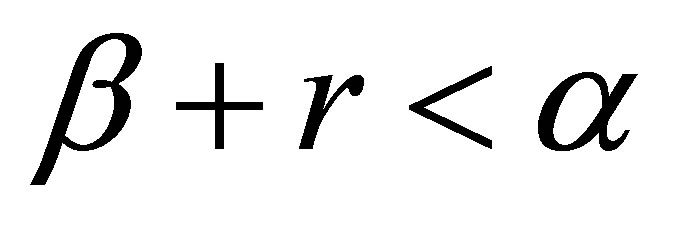 . Let
. Let  be the eigenvalue of
  such that
 , and
, and
 a corresponding eigenfunction:
Set . As easily seen from Equation (29), the function
  given by
is the solution to Equation (9) with the initial value . In view of the reduction process to Equation (30), the function
  is thus a non-trivial solution to (30). This shows that the decay (31) for
  is no longer improved. This finishes the proof of Theorem 4. Q.E.D.
Example. In (1), let us consider the case where  is a bounded interval
 . The pair of differential operators
  is then rewritten as
 (36)
(36)
where , and
, and . Let
. Let  be an operator defined, for
 , by
, by
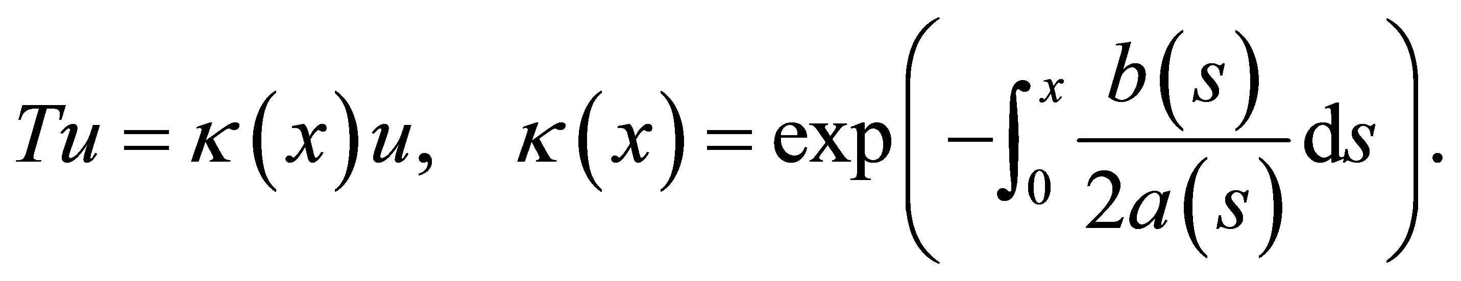
Clearly  defines an isomorphism in
 . Let us consider the case where
  is of the third kind, i.e.,
 . Then,
  transforms
  into another pair
 , which defines a self-adjoint operator
  with dense domain
 . In
. In ,
,  is unchanged;
  and
and  are changed, respectively, to 0 and
 ; and
; and  of the third kind. The idea is a slightly modified version of the well known result (see page 292 of [18]). Based on this, we have
Proposition 6. 1) The spectrum  consists of real and simple eigenvalues:
 ,
,
 .
.
2) The eigenfunctions  of
of  forms a Riesz basis. Any
  is uniquely expressed as
 .
.
In our problem, we know that ,
, . Thus we choose
 , so that the output of the system is a single observation at the end point
  as
as
 (37)
(37)
that is,  ,
, . Let us examine some assumptions in Theorem 4 in this example. Most important is the complete observability (18). The matrices
  in (16) are now
 ,
, . Thus, we see that the complete observability is satisfied. Since
  in (13) is a one dimensional operator, the multiplicities of the eigenvalues
  are equal to 1. This enables us to choose
  in (9). In Proposition 3, the controllability condition on the actuator
  is stated as follows: let
  be eigenfunctions of
 . By setting
 , the controllability condition is simply that
 ,
,  ,
, .
.
In the case where  is of the first kind, the output is a single observation at the end point
  as
as . Proposition 6 also holds in this case. Since
 ,
,  , the complete observability is similarly satisfied.
3. Spectral Property of the Coefficient Operator
We go back to the problem raised in Section 1: Unlikeliness of a vector of the form . The basic control system is Equation (30) in the product space
 . To avoid any unnecessary technical complexity, we limit ourselves to the simple case of one dimensioanl equations raised in (36),
  being of the third kind. In the setting of the space
  as well as
  in (6), we can choose
 ,
, . Thus,
 . Equation (30) is simply rewritten as
 (38)
(38)
where  is defined as
 (39)
(39)
and . Here,
  (see
(see
(37)). The operator  is sectorial, and every solution to (30) or (38) is expressed as
 ,
, . Let
. Let  be the projector corresponding to a
  with
with . In view of the relation:
the right-hand side of which decays as  with decay rate
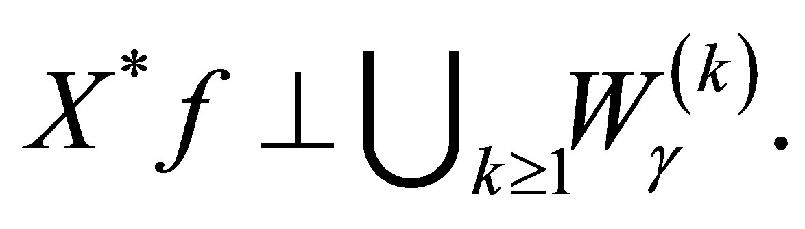
  for every initial state. Now we ask: Does the range of the
  contain a vector of the form
 ? This problem immediately leads to the structure of the eigenspaces of the operator
 . In the operator
 , the vectors
  and
and  of the compensator are the parameters to be designed
 . In designing these parameters, they are generally influenced by small perturbations. It is thus implausible to assume that some Fourier coefficients of these parameters would be designed to be
 : such conditions are very easily broken. Thus we may henceforth assume that
 (40)
(40)
where  and
and  denote, respectively,
and . The actuators
  and
and  of the controlled plant are the given parameters in advance. It is also implausible to assume that some Fourier coefficients of
  and
and  relative to
  might be equal to 0. Thus we may also assume that
 (41)
(41)
The main results in this section are Theorem 7, Proposition 8, and Theorem 9 stated just below. The proof of these results will be given later.
Theorem 7. Let . Suppose that
  and that
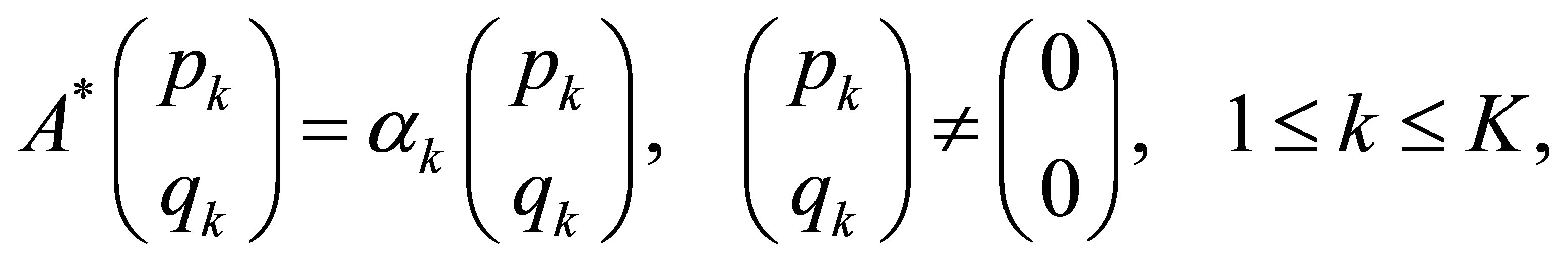 (42)
(42)
where 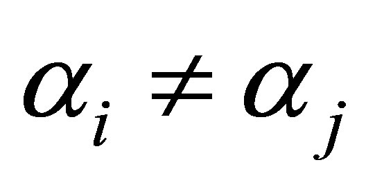 for
for . Then any linear combination of these eigenvectors
  of
of  cannot generate a vector of the form,
  ,
, .
.
Remark. The adjoint operator  will be characterized later in (49). Theorem 7 also asserts that there is no eigenvector of the form,
  ,
, . The restriction on
  is derived from our setting of the operator
  in (39): The setting is made for constructing a finitedimensional compensator. In the original equation (9), however, the parameters are constructed in a more general setting. The operator
  is then replaced by
 (39')
(39')
Then, the above restriction on the  is removed: In fact, the integer
  may be chosen arbitrarily large.
We hope to know more on . The following proposition partly gives concrete informations on what
  consists of. It shows that
  is contained in
 , regardless of the assumptions (40) and (41).
Proposition 8. The numbers ,
,  belong to
 . Actually we have the relations:
 (43)
(43)
for . Since the set
  forms an orthonormal system for
 , any linear combinations of these eigenvectors cannot generate a vector of the form,
  ,
, .
.
To seek eigenvalues of  other than
 , let us recall the operator
  which appeared in (32), where
 with
with 
 . The adjoint operator
  is clearly given by
 with
with 
In the following result, we characterize  by introducing an operator
 , a slightly perturbed operator of
 :
:
Theorem 9. Let  be an operator defined as
 (44)
(44)
where . Then, we have the relation
 (45)
(45)
Let  be an arbitrary eigenpair of
  such that
  is not contained in
 . Then, the corresponding eigenvector
  of
of  is given by
 (46)
(46)
where .
.
In the above assertions, we need to characterize the adjoint operator , which will be described later by (51). To seek the structure of
 , let us begin with the operator equation:
 (47)
(47)
It is clear that (47) admits a unique solution , and that the solution is expressed as
  (see (17)). Let
  be a unique solution to the boundary value problem:
  in
in ,
,  on
on . We note that
  remains bounded when
  (this fact will be used in Lemma 10 below). For any
 , note that
Then the adjoint  is expressed as
where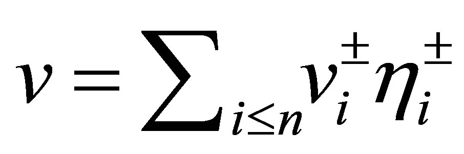 ,
, . Thus,
 (48)
(48)
Let us find the equation for . For
. For  and
and , we calculate through Green’s formula, (47), and the boundary condition (48) as
and thus . Since
  is dense in
 , we see that
 (49)
(49)
Let us calculate the adjoint . By assuming that
  is in
is in  and satisfies the boundary condition:
 ,
,  is calculated as
where  is given by
 (50)
(50)
and 
 We see that
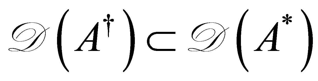 , and thus
 . In order to show that
 , we need the following elementary result:
Lemma 10. The operator  is densely defined, and the bounded inverse,
 exists for a sufficiently large
 .
.
Proof. Given a , we solve the equation:
 , where
 . Set
. Set , and define an operator
  as
as
The function  depends on
 . However, since
  remains bounded as
 , there is a bounded inverse:
  for a sufficiently large
 . A straightforward calculation shows that
  defined by
  and
and 
 uniquely solves the above equation. Thus the bounded inverse
  exists.
Denseness of : it is enough to show that
implies . The above left-hand side is calculated for every
  as
as
Since  is dense, this means that
and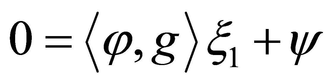 , from which we conclude that
 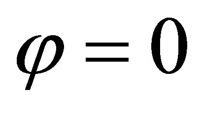 and
and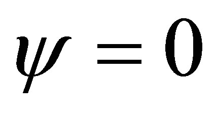 . Q.E.D.
In view of the fact that both  and
and  exist as a bounded inverse, it is immediate that
  is contained in
 . We have proven that
 (51)
(51)
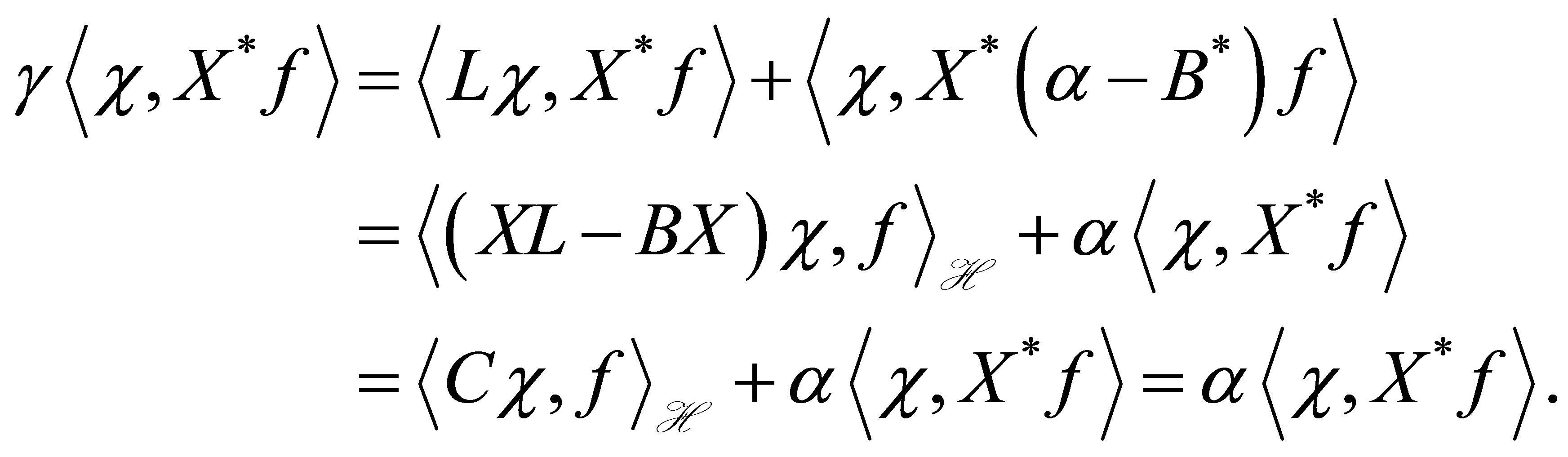
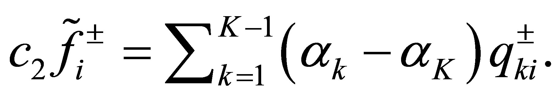
Proof of Proposition 8. By setting  and
and ,
,  ,
,  belongs to
 . By (49), we see that
 , and
, and 
 , which shows (43) Q.E.D.
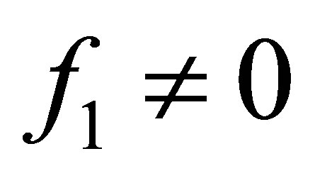
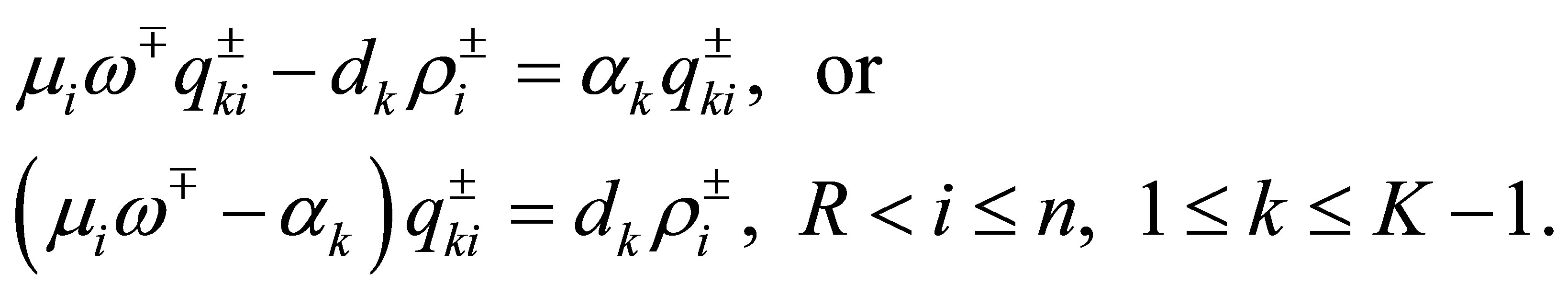
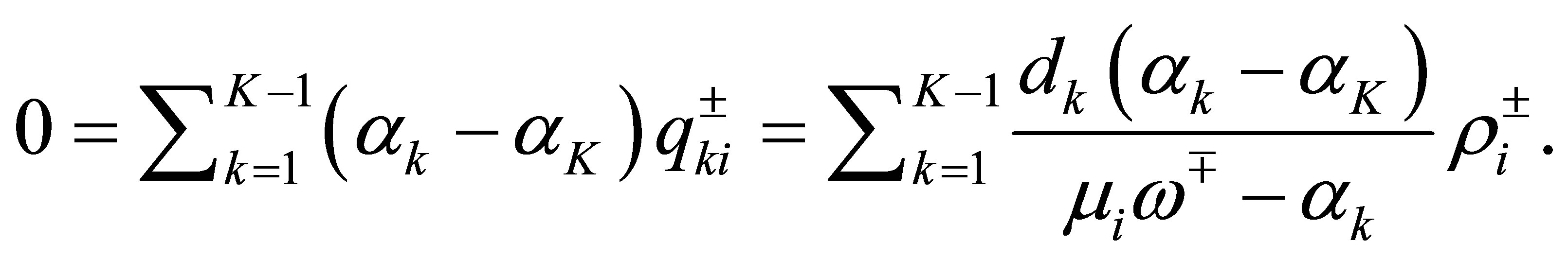
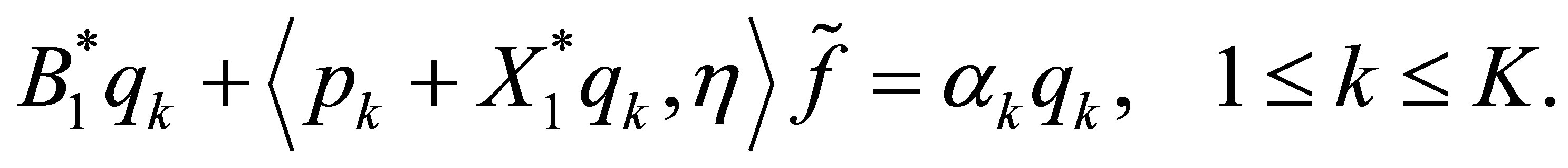
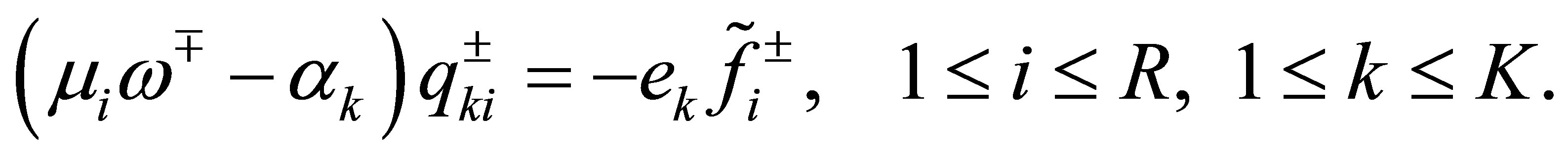
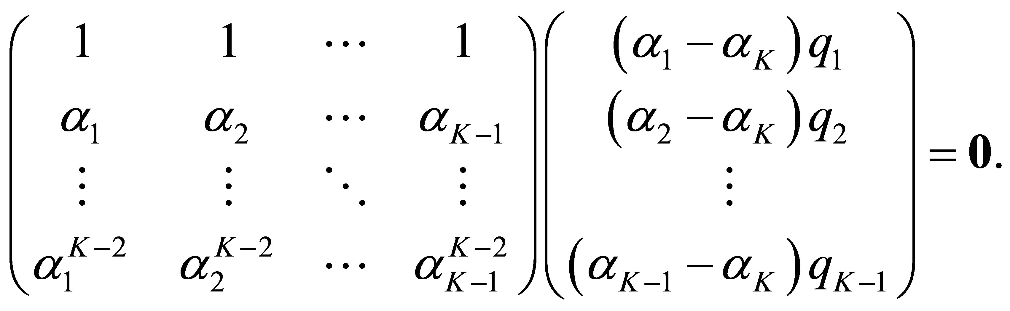
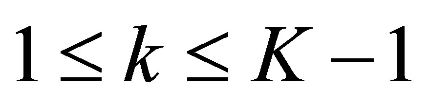
Proof of Theorem 7. Assuming that  in (42), we derive a contradiction. In (42), adding the equations of
  over 1 through
 , we see that
 (52)
(52)
where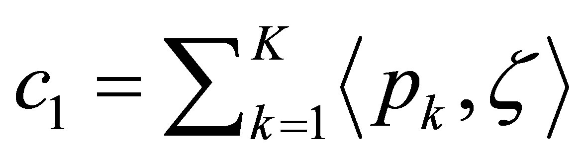 ,
,  , and
, and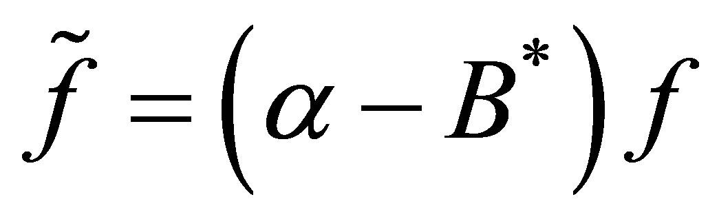 . The Fourier coefficients of these vectors relative to the orthonormal system
  satisfy
 (53)
(53)
where . Note that
 for
for . We show that
 . Supposing the contrary, we must have
 (54)
(54)
Set ,
,  for simplicity. Then,
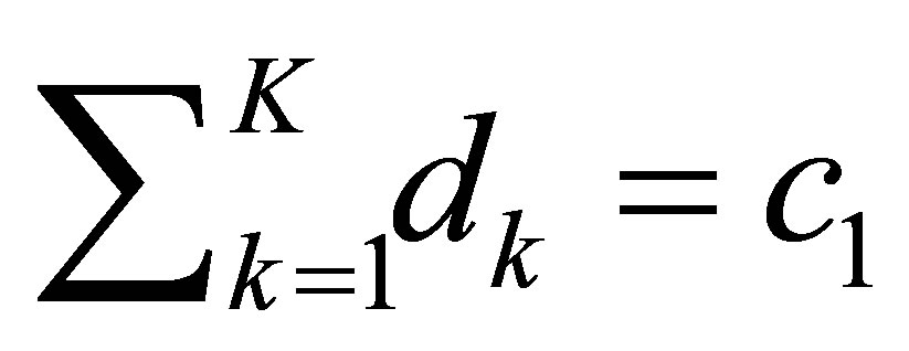 . In the equation for
 ,
, 
 , we see that
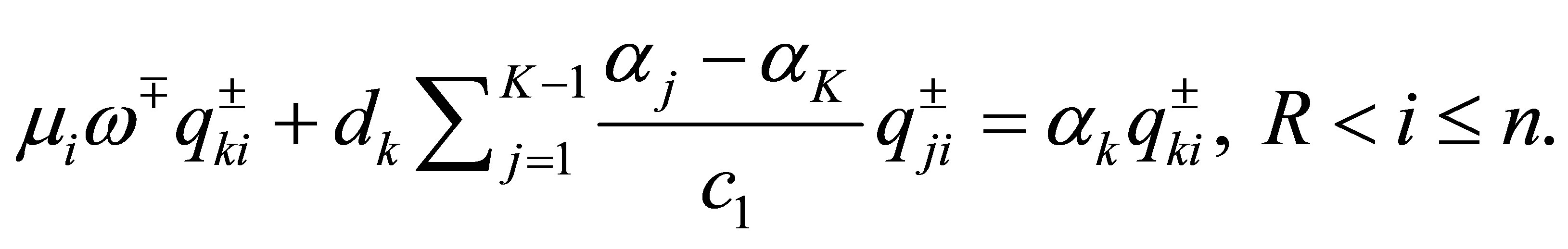
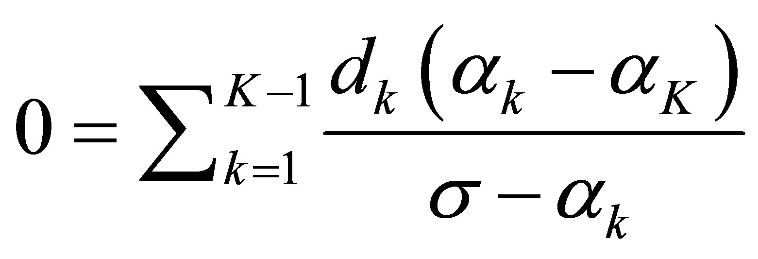
The number of these  is
is . Consider the algebraic equation in
 :
:
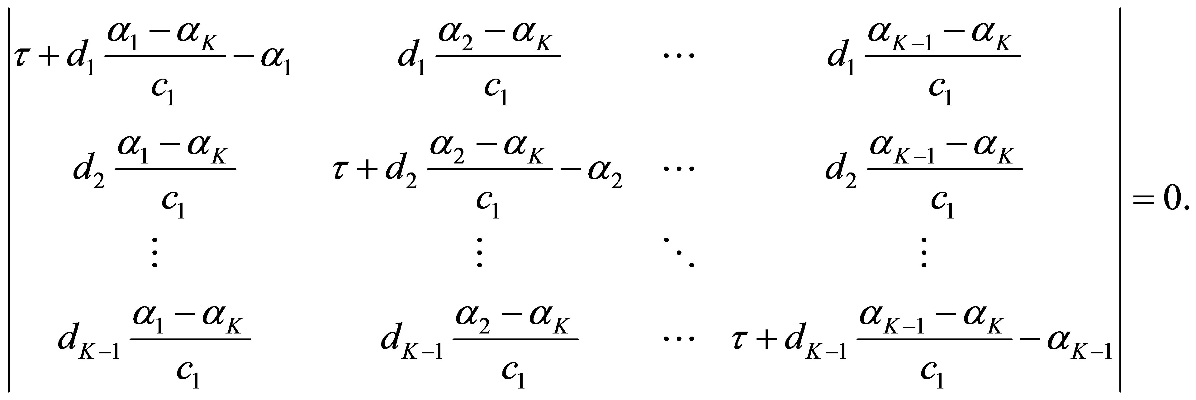
The equation admits  solutions. The number of the solutions
  which agree with one of the
  is at most
 . In other words, the determinant is not equal to 0 for the other
 , the number of which is atleast
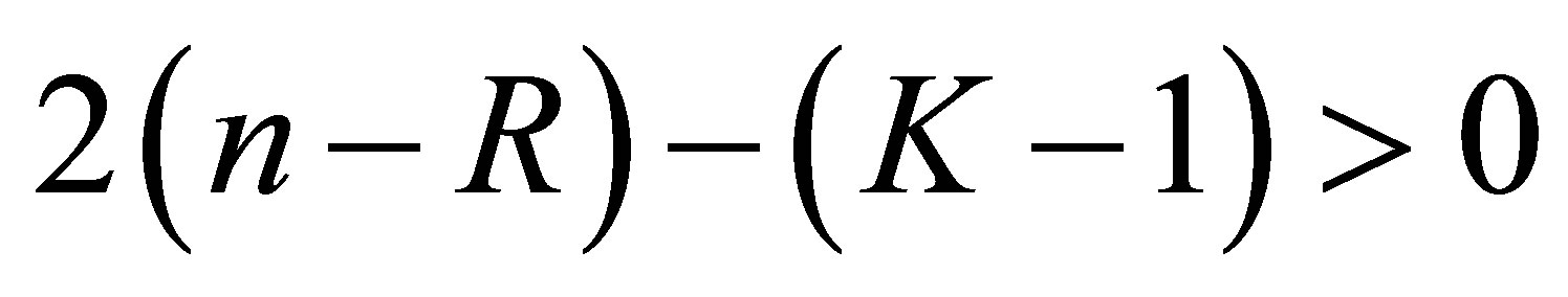 . Thus for these
 , we must have
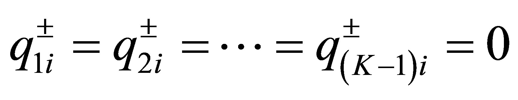 . By (53), this implies that
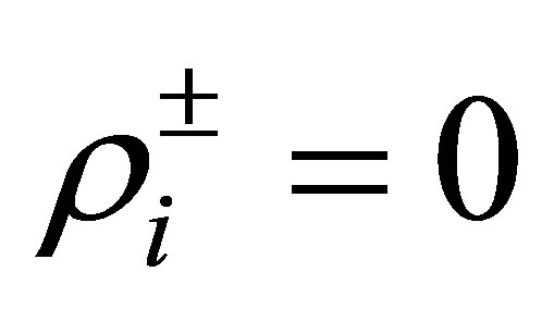 , which contradicts our assumption (40). We have shown that
 . Thus we have, for
 ,
,
 (55)
(55)
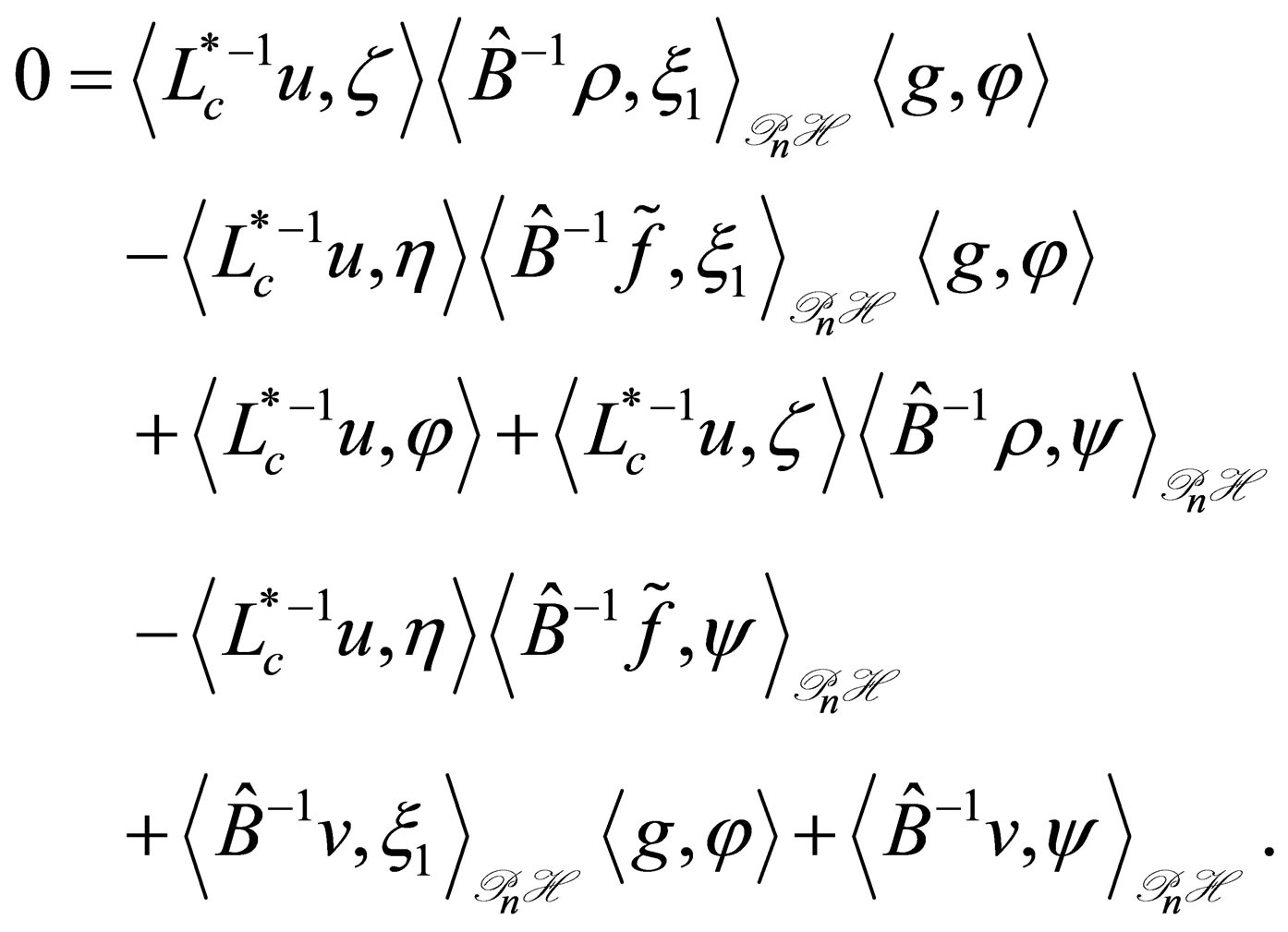
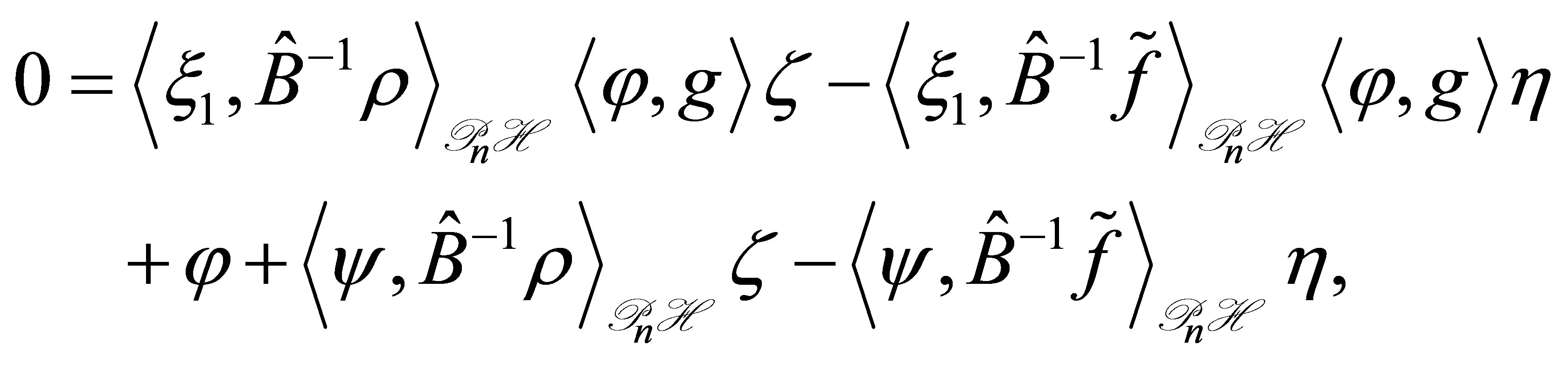
Comparing the Fourier coefficients in the equations to  in (42), we see that
The number of the eigenvalues  which agree with one of the
  is at most
 . In other words, the number of the
  which does not agree with any of the
  is at least
 . For these
 , we see from (55) that
Since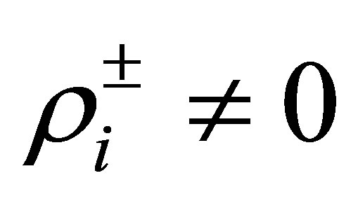 , this means that the relation in
 :
:
 (56)
(56)
holds for the above , the distinct number of which is at least
 . This implies that the relation (56) holds for any
 . calculating the residue at each
 , we find that
 , and thus
 , too.
We go back to the equations to  in (42) again. Since
 ,
,  , we have
Set . Then,
 . Calculating the Fourier coefficients, we have
The numbers of these  and
and  are
are  and
and , respectively. Thus, the number of
  which does not agree with any of
  is at least
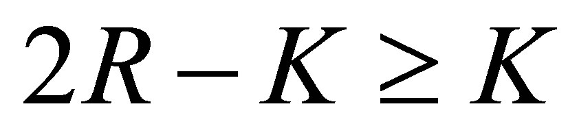 . For these
 , we see by the relation (54) that
But, since  by (40), this means that the relation in
 :
:
 (57)
(57)
holds for the above , the distinct number of which is at least
 . The situation is the same as in (56). Thus the relation (57) holds for any
 . Calculating the residue at each
 , we similarly find that
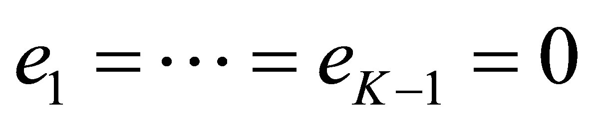 ,
,  , and thus
 , too. Since
 ,
,  , we have finally obtained from (42) and (55) that
 ,
,  , and
, and
 . Applying
  to the both sides of the above second equation, we see that, for
 ,
,

In other words, we have the relation:
But  for
for . Thus, we immediately find that
 ,
,  , i.e.,
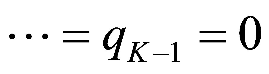
 , and that
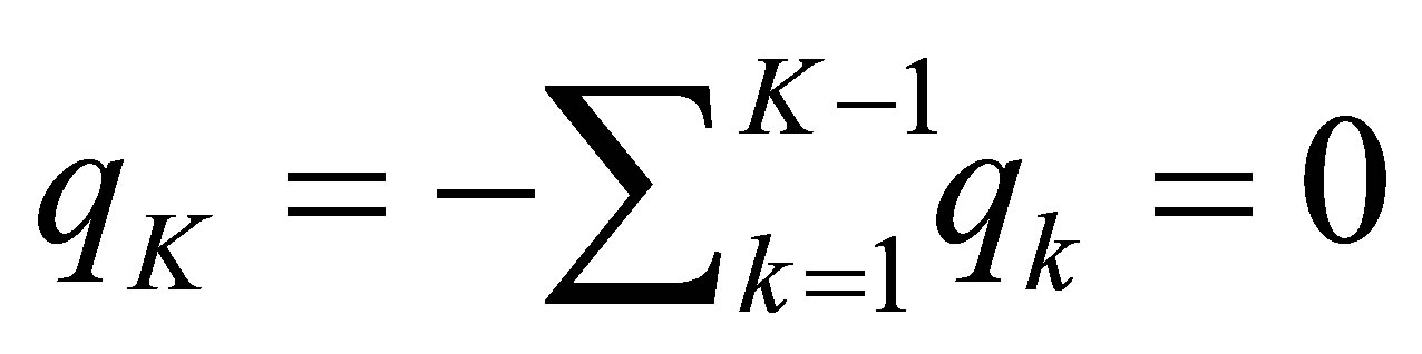 .
.
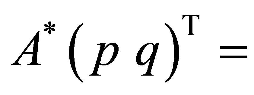
Recall that ,
, . Thus,
  belongs to
 , and
, and 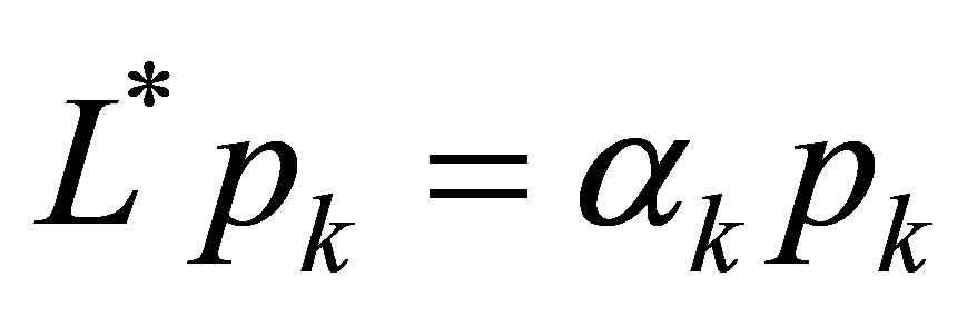 by (42). Each
  is found an eigenvalue of
 , and
, and  must be an eigenfunction. In addition,
But, this contradicts our assumption (41). Q.E.D.
Proof of Theorem 9. We already know that 
 by Proposition 8. Let
  be in
be in .
.
In view of (51), the relation: ,
,  means that
 (58)
(58)
where . The calculation of: (the first equation) +
  × (the second equation) yields that
By noting that 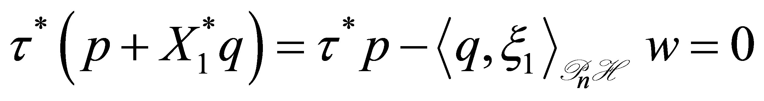 (see (48)), the function
 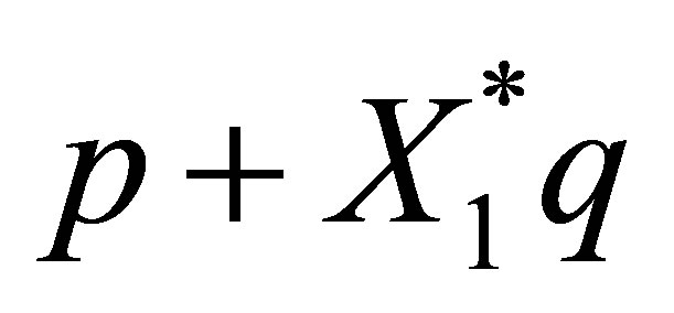 belongs to
 . Thus we see that
 . Supposing that
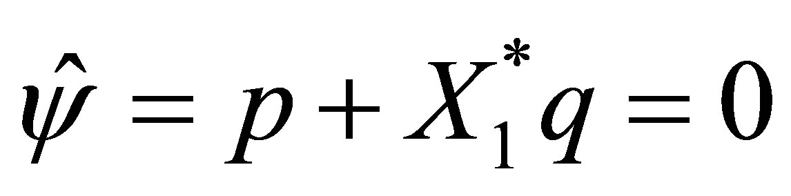 , we show a contradiction. In fact, if so, the second equation of (58) becomes
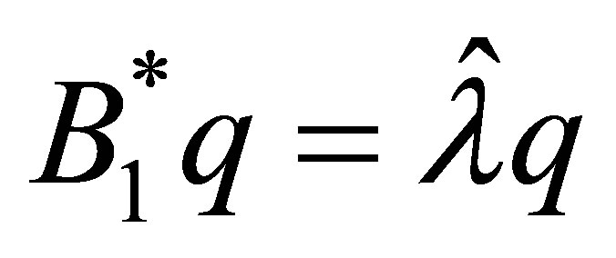 . Since
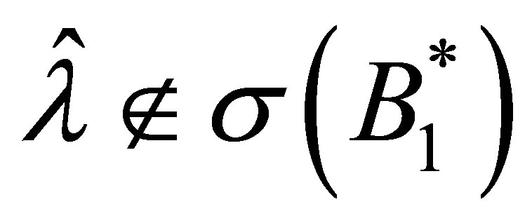 , however, we see that
 , and
, and , or
, or . Thus,
  belongs to
 , and the corresponding eigenvector of
  is given by the form
 , where
 . We have also shown that
 .
.
Conversely, let  be an arbitrary eigenpair of
  such that
 . Then we solve the equation:
 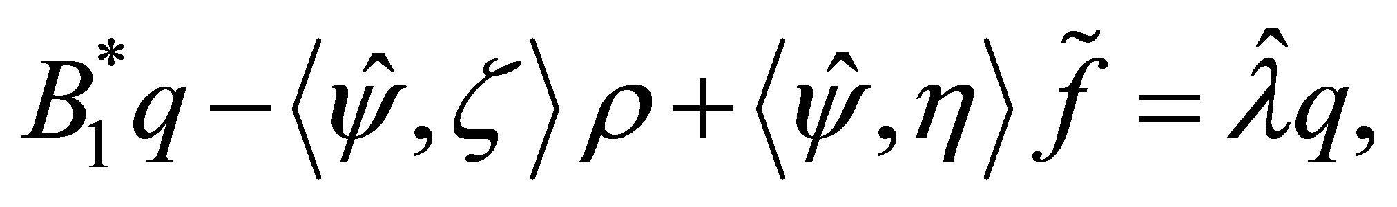 the unique solution of which is given by
 .
.
By setting , the vector
  means (46), and clearly satisfies the relation:
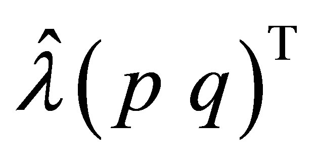
 .To show that
 , we suppose the contrary:
 , or
, or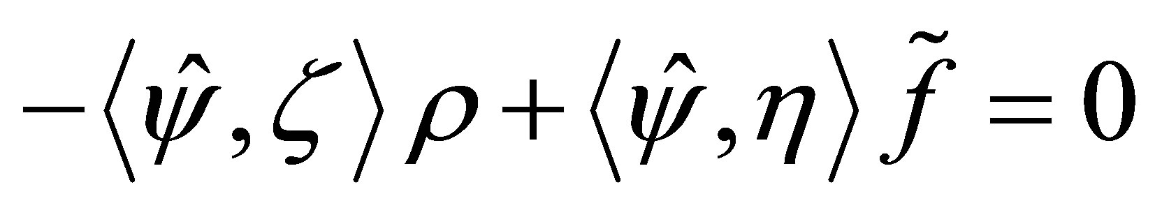 . Then,
  , and
, and . Thus,
  must be an eigenpair of
 . But, this contradicts the assumptions (40) and (41). We have shown that
  given by (46) is an eigenvector of
 . Q.E.D.
Remark. In (45), it is not certain if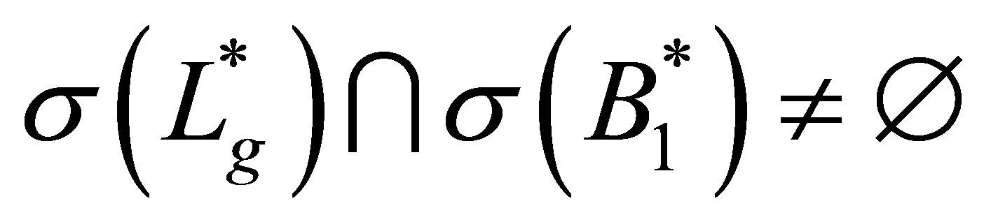 . This problem seems a pathological one. If
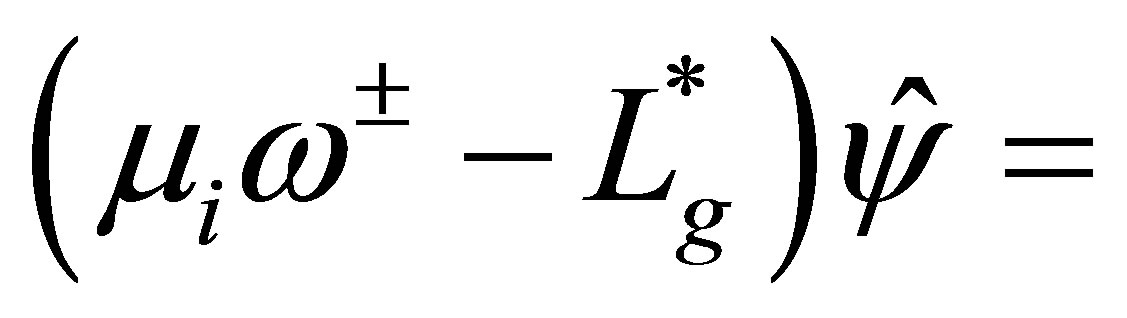
 ,
,  for some
 ,
,  , and, in addition,
  , then the equation
 admits a (non-unique) solution
  (see the second equation of (58)). By setting
 , the vector
  belongs to the eigenspace of
  for
for .
.
NOTES