1. Introduction
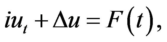
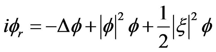
We consider the Cauchy problem for the nonlinear Schrö- dinger equation in dimension d = 2.
 (1.1)
(1.1)
where ,
,  , and
, and , When
  (1.1) is called defocusing when
  (1.1) is called focusing. In this paper we discuss the case when
  and
and  (defocusing case).
If  is a solution to (1.1) on a time interval
  then
then
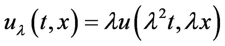 (1.2)
(1.2)
is a solution to (1.1) on  with
with .
.
This scaling saves the  norm of u,
 (1.3)
(1.3)
Thus (1.1) under previous hypotheses is called L2-critical or mass critical.
Proposition 1.1. Suppose that  and
and 
then, for any initial data , there exist
  such that there exists a unique solution
of the nonlinear Schrödinger Equation (1.1). If  then
then  for some non-increasing, and if
  is sufficiently small u exists globally.
In this paper we will discuss the case, 
This means that a solution u
 and called critical solution.
Definition 1.1. Let ,
,  is a solution to (1.1) if for any compact
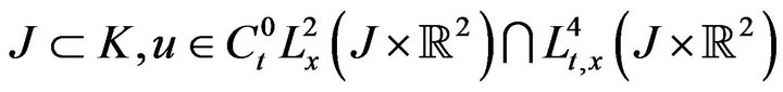
and for all 
 (1.4)
(1.4)
The space 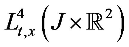 caused from strichartz estimates. This norm is invariant under the scaling (1.2).
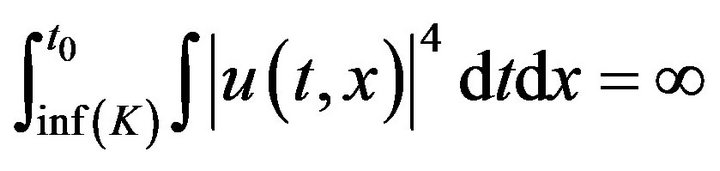
Definition 1.2. If there exist  a solution u to (1.1) defined on
  blows up forward in time, such that
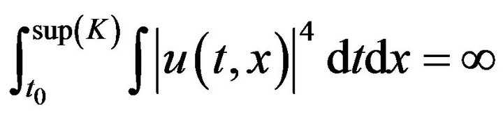 (1.5)
(1.5)
And u blows up backward in time, such that
 (1.6)
(1.6)
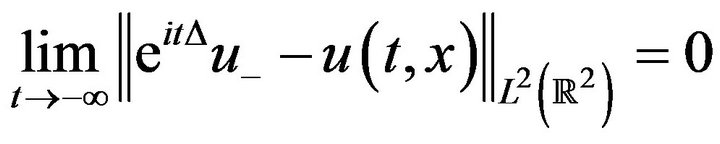
Definition 1.3. If there exist  we say that a solution u to (1.1) scatter forward in time such that,
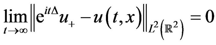 (1.7)
(1.7)
A solution is said to scatter backward in time if there exist 
Such that,
 (1.8)
(1.8)
We note that the Equation (1.1) has preserved quantities, the mass
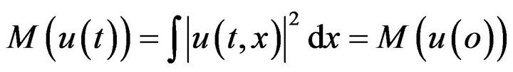 (1.9)
(1.9)
And energy
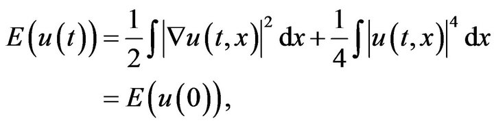 (1.10)
For more see [1].
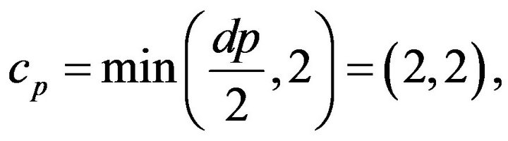
Proposition 1.2. let p be the  -critical exponent
 , then the NLS (1.1) is locally well posed in
 in the critical case. More precisely, given any
 , there exists
  such that whenever
  has norm at most R, and K is a time interval containing 0 such that
Then for any u0 in the ball

there exists a unique strong  solution
  to (1.1), and moreover the map
 , is Lipschitz from B to
 , where
  defined in Equation (2.5).
Proposition 1.3. let K be a time interval containing  and let
  be two classical solutions to (1.1) with same initial datum u0 for some fixed μ and p, assume also that we have the temperate decay hypothesis
  for q = 2, ∞. Then
 .
.
Proposition 1.4. Let , given
  there exists a maximal lifespan solution u to (1.1) define on
 , with
 . Furthermore1) k is an open neighborhood of
 .
.
2) We say u is a blow up in the contrast direction If  or
or  is finite.
3) If we have compact time intervals for bounded sets of initial data, then the map that takes initial data to the corresponding solution is uniformly continuous in these intervals.
4) We say that u scatters forward to a free solution, if  and u does not blow up forward in time. And we say that u scatters backward to a free solution, if
  and u does not blow up backward in time.
To Proof: see [1-3].
2. Strichartz Estimates
In this section we discuss some notation and Strichartz estimates for critical NLS (1.1) and we turn to prove Propositions 1.1 and 1.3.
2.1. Some Notation
If X, Y are nonnegative quantities, we use  or
or , to denote the estimate
  for some c and
  to denote the estimate
We defined the Fourier transform on  by
by
We use  to denote the Banach space for any space time slab
  of function
  with norm is
With the usual amendments when q or r is equal to infinity. When  we cut short
  as
as .
.
Defined the fractional differentiation operators ,
,  by
by

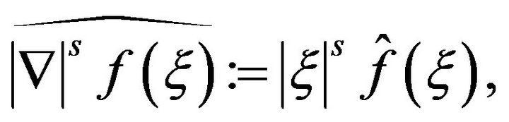
where , specially, we will use
  to signify the spatial gradient
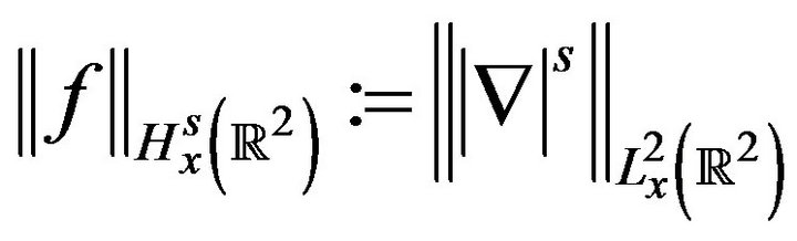
  and define the Sobolev norms as

Let  be the free Schrödinger propagator; in terms of the Fourier transform, this is given by,
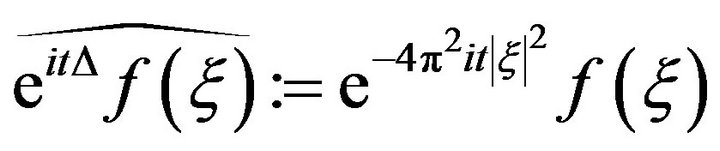 .
.
A Gagliardo-Nirenberg type inequality for Schrödinger equation the generator of the spurious conformal transformation 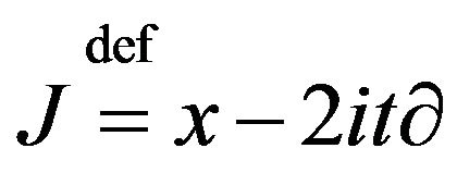 plays the role of the partial differentiation.
2.2. Strichartz Estimates
Let  be the free Schrödinger evolution, from the explicit formula
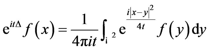 (2.1)
(2.1)
Specially, as the free propagator saves the  -norm,
For all  and
and , where
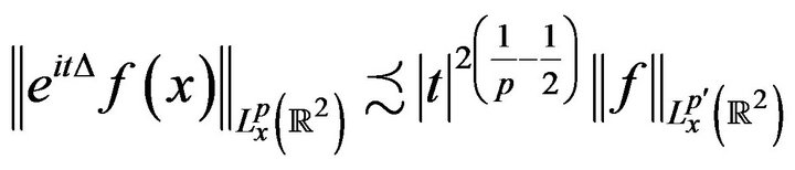
Proposition 2.1. There holds that
 (2.2)
(2.2)
In fact, this follows directly from the formula (2.1).
Definition 2.1. Define an admissible pair to be pair
 with
with ,
,  , With
Theorem 2.2. If  solves the initial value problem
 On an interval K, then
 (2.3)
(2.3)
For all admissible pairs ,
, .
.  denotes the Lebesgue dual
 .
.
To prove: see [4,5].
Definition 2.2. Define the norm
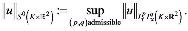 (2.4)
(2.4)
 (2.5)
(2.5)
We also define the space  to be the space dual to
  with suitable norm. By theorem.2.2,
 (2.6)
(2.6)
Theorem 2.3. If  is small, then (1.1) is globally well posed, for more see [6,7].
Proof: by (2.3) and (2.6)
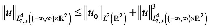 (2.7)
(2.7)
If  is small enough and by the continuity method, then we have global well-posedness. Furthermore, for any
  there exist
  such that

Then
 (2.8)
(2.8)
So by (2.6), when 
 (2.9)
(2.9)
Thus, the limit
 (2.10)
Exists, and,
 (2.11)
A conformable argument can be made for 
indeed, if , then
  can be division into
  subintervals K with
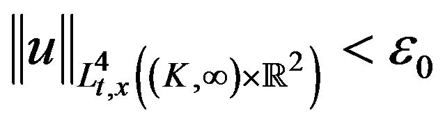
on each subinterval. Using the Duhamel formula on each interval individually, we obtain global well-posedness and scattering. 
Now we return to prove Proposition 1.1 and Proposition 1.3.
Proof proposition 1.1:
We suppose in what follows that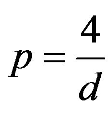 . Let
. Let
 and for some
  to be chosen,
 be such that
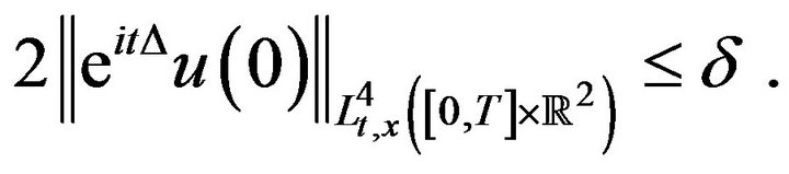 (2.12)
We deem the space
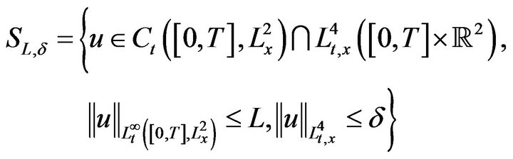
And the mapping,
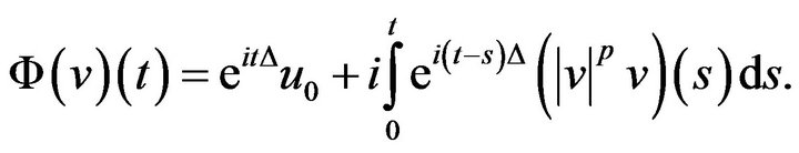 (2.13)
We want to prove that the δ small adequate, 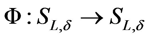 is contraction. We use first Strichartz estimates, to compute that

where 
Then, distinctly,

So that for  is small enough,
  is settled under
 . In addition,

Again, decreasing may be , we get a contraction.
If , then
 , and from Strichartz estimateswe see that if
  is small enough, then (2.12) is satisfied for

Proof Proposition 1.3: By time translation symmetry we can take . By time reversal symmetry we may assume that K lies in the upper time axis
 . Let
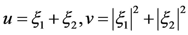
. Let , and then,
  ,
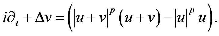
,  and v obey the variance equation
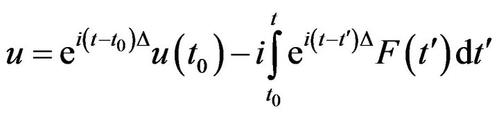
Since v and  lies in the
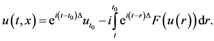
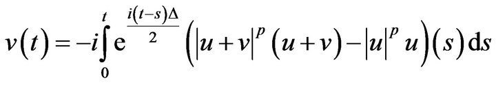
  we may calling Duhamel’s and conclude
for all. By Minkowski’s inequality, and the unitarity of , conclude that,

Since u and v are in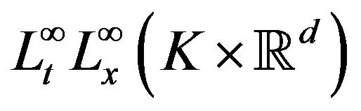 , and the function
  is locally Lipcshitz, we have the bound
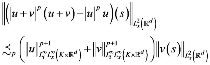
Apply Gronwall’s inequality to conclude that
 for all
  and hence
 .
. 
3. Decay Estimates
Consider the defocusing nonlinear Schrödinger Equation (1.1), in , where
  and
and , for
, for . We suppose that at
 (3.1)
(3.1)
First we have the following result.
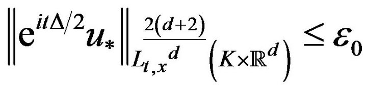
Theorem 3.1. Suppose that , if
, if  and let u be a solution to (1.1), identical to an initial data
 such that
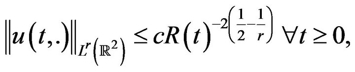
 . If d = 2let r be such that,
  , then there exists a constant c > 0 such that if R is the solution of,
 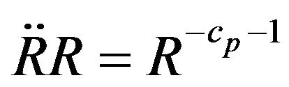 , with
 ,
,  then
then
Furthermore, c depends only on d, p, r and,
 .
.
The method made up in rescheduling, by the average of a time dependent rescheduling the equation, and to use the energy of the equation, to get by interpolation decay estimates in suitable norms. The asymptotically average, is normally obtained directly by using the pseudo conformal law, the above result was in fact partially proved in [8], under a bit different point of view: look for a time dependent change of coordinates, which maintain the Galilean invariance, and the construction directly a Lyapunov functional by a suitable ansatz. This Lyapunov functional is surely the energy of the rescaled equation. Our aim here is to study with further details the rescaled wave function and its energy. Found to be the method provides rates which are seems completely new in the limiting case of the logarithmic nonlinear Schrödinger equation. Because of the reversibility of the Schrödinger equation and standard results of scattering theory, one cannot foresee the convergence of the rescaled wave function to some a intuition given limiting wave function, but found to be some convexity properties of the energy can be used to state an asymptotically stabilization result. From the general theory of Schrödinger equations, it is well known that the Cauchy problems (1.1)-(3.1) is well posed for any initial data in  when
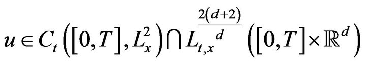
when , and that the solution u belongs to
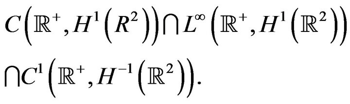
As usual for Schrödinger equations is critical when .
.
Let  be such that
 .
.
where and  are positive derivable real functions of the time.
It is simple to check that with this change of coordinates,  satisfies the following equation,
where , with the choice
 , which means that
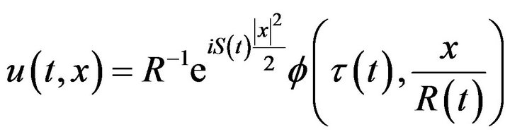
  and u are linked by,
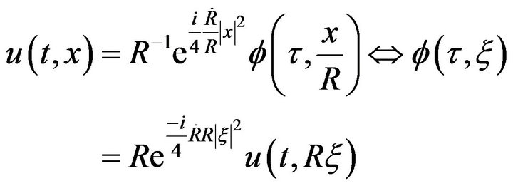 (3.2)
(3.2)
where  and
and 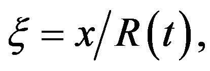 and
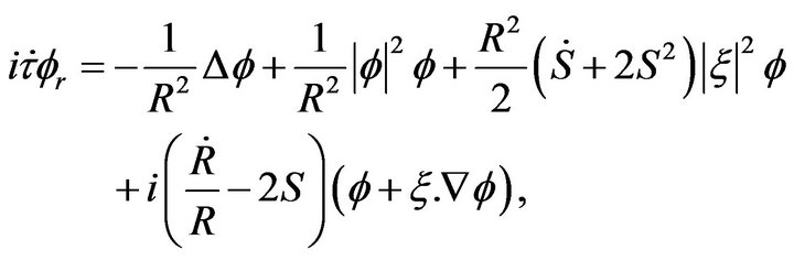
and  has to satisfy the following time-dependent defocusing nonlinear Schrö- dinger equation,
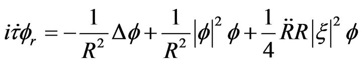 (3.3)
(3.3)
We note that 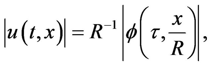 so that

for all .
.
Also we note that if  and
and  then
then
 (3.4)
(3.4)
To extract the controlling impacts as  we fix
  and R such that,
where
 (3.5)
(3.5)
Because p is critical, this ansatz is actually the only one that sets to 1 at least three of the four coefficients in the equation for , with
  and
and  solves the equation,
 (3.6)
(3.6)
With the choice  and
and , integration of (3.5) with respect to t gives
 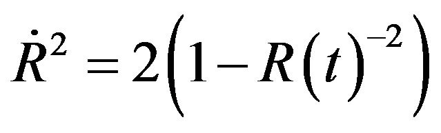 and this is possible if, and only if,
  for all
  thus the function
  is globally defined on
  increasing,
  and
and  as
as .
.
Supposing that ,
,  is an increasing positive function such that,
 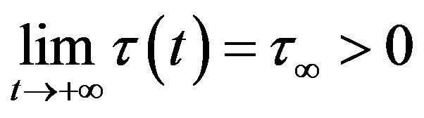 , where
  if
if .
.
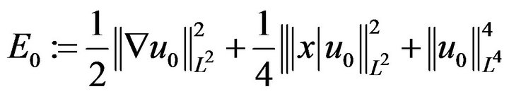
Consider now the energy functional linked to Equation (3.6)
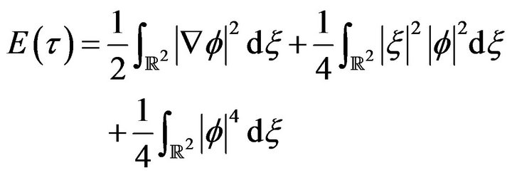 (3.7)
(3.7)
where R has to be understood as a function of.
Lemma 3.2. Suppose that , if
, if , and let u be a solution to (1.1), identical to an initial data,
 such that
 .
.
With the above notations, E is a decreasing positive functional. Thus  is bounded by
 , with the notations of Theorem 3.1.
Proof: The proof follows by a direct computation.
Because of (3.6), only the coefficients of , and
, and  contribute to the decay of the energy.
For more see [9]. 
Proof of Theorem 3.1: Suppose that p is critical. By Lemma 3.2 and pursuant to the time-dependent rescaling (3.2),

Thus

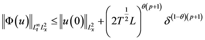
Is bounded by , the remainder of the proof follows the same lines that in Theorem 7.2.1 of [10], see also [11,12], using maintain the L2-norm and the Sobolev-Gagliardo-Nirenberg inequality.
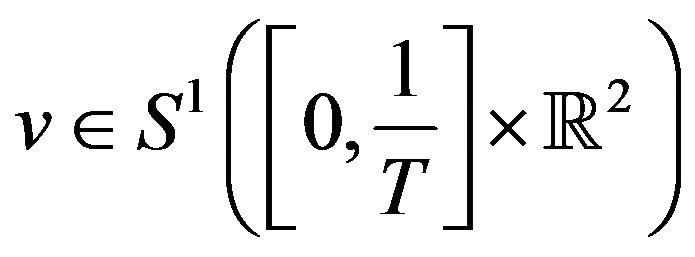
Proposition 3.3. Consider the two-dimensional defocusing cubic NLS (1.1), (is  -critical). Let
  then there exists a global
  -well posed solution to (1.1), and moreover the
  norm of u0 is finite.
Proof: By time reflection symmetry and adhesion arguments we may heed attention to the time interval  Since u0 lies in
 , it lies in
 . Apply the
  well posedness theory (Proposition 1.2) we can find an
  -well posed solution
 , on some time interval
  with
with  depending on the profile of u0.
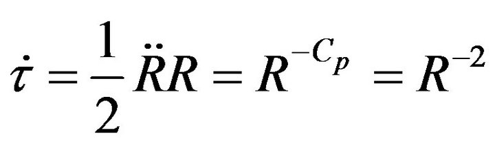
Specially the  norm of u is finite. Next we apply the pseudoconformal law to deduce that,
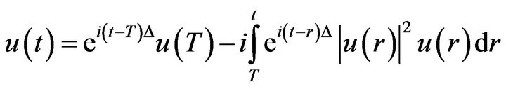
Since , we got a solution from t = 0 to t = T. To go to all the way to
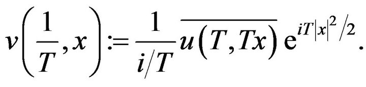
 . We apply the pseudoconformal transformation at time t = T, obtaining an initial datum
  at time
  by the formula
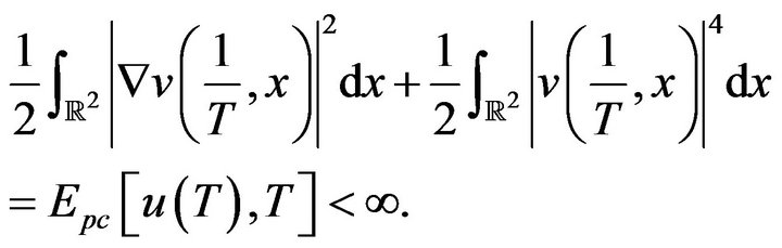
From 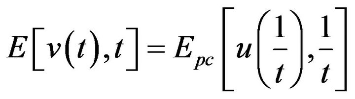 we see that v has finite energy:
And, the pseudoconformal transformation saves mass and hence

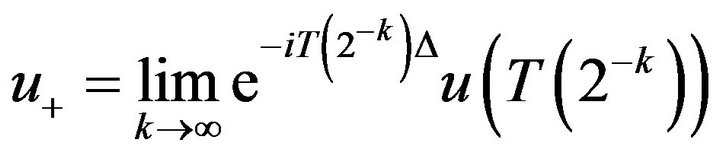
So we see that  has a finite
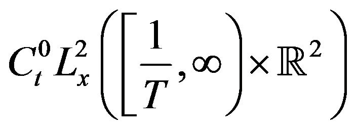
  norm. Thus, we can use the global
  -well posedness theory, backwards in time to obtain an
  -well posed solution
 , to the equation
 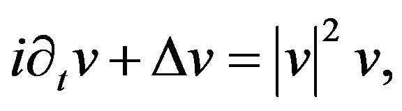 particularly,
We reverse the pseudoconformal transformation, which defines the original field u on the new slab 
 We see that the
 , and
, and
 norm of u are finite. This is sufficient to make u an
  -well posed solution to NLS on the time interval
 ; for v classical. And for general
 , the claim follows by a limiting argument using the
  -well posedness theory. Adhesion together the two intervals
  and
and , we have obtained a global
  solution u to (1.1).
4. Some Lemma
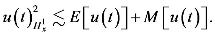
Consider the defocusing case of the NLS (1.1) and if , the energy and mass together will control the
  norm of the solution:
Conversely, energy and mass are controlled by the  norm (the Gagliardo-Nirenberg inequality showed that):
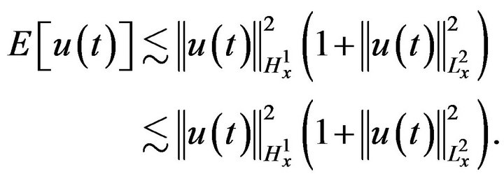

This bound and the energy conservation law and mass conservation law showed that for any  -well posed solution, the
  norm of the solution
  at time t is bounded by a quantity depending only on the
  norm of the initial data.
Proposition 4.1. The cubic NLS (1.1) with , d = 2 is globally well posed in
 . Actually, for
  and any time interval, K the Cauchy problem (1.1) has a
  well posed solution
Lemma 4.2. If  the following holds:
 .
.
Proof: The proof depends on the noticing that;
 .
.
With
Thus
By standard Gagliardo-Nirenberg inequality,
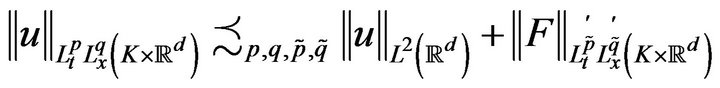
Lemma.4.3. Let . For any spacetime slab
 ,
,  , and for any
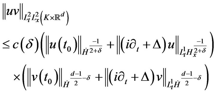 (4.1)
(4.1)
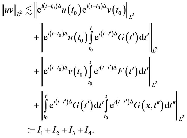
The estimate (4.1) is very helpful when u is high hesitancy and v is low hesitancy, as it moves abundance of derivatives onto the low hesitancy term. In particular, this estimate shows that there is little interaction between high and low hesitancy. This estimate is basically the repeated Strichartz estimate of Bourgain in [13]. We make the trivial remark that the  norm of uv is the same as that of
 ,
,  , or
, or , thus the above estimate also applies to expressions of the form
Proof: We fix , and permit our tacit constants to depend on
 . We begin by dealing with homogeneous case, with
  and
and , And consider the more general problem of proving,
 (4.2)
(4.2)
where  the scaling invariance of this estimate, first, our objective is to prove this for
  and
and .
.
May be recast (4.2) using duality and renormalization as
 (4.3)
(4.3)
Since , we may restrict attention to the interactions with
In fact, in the residual case we can multiply by
 to return to the condition under discussion. In fact, we may further restrict attention to the case where
  since, in the other case, we can move the frequencies between the two factors and reduce the case where
 , which can be dealt by
  Strichartz estimates when
  Next, we decompose
  dyadically and
  in dyadic multiples of the size of
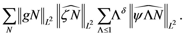
  by rewriting the quantity to be controlled as (N,
  dyadic):

Note that subscripts on  have been inserted to invoke the localizations to
 ,
,  ,
,  , consecutive. In the case
 , we have that
  and this expound, why g may be so localized. By renaming components, we may suppose that
  and
and .
.
Write  We change variables by writing
And 
We show that by calculation
Thus, upon changing variables in the inner two integrals, we encounter

where
Apply the Cauchy-Schwarz on the u, v integration and change back to the original variables to obtain
We recall that  and use Cauchy-Schwarz in the integration, taking into consideration the localization
 , to get
Choose  and
and . with
  to obtain
This summarizes to get the claimed homogeneous estimate. Now we discuss the inhomogeneous estimate (4.1). For simplicity we set,  and
and  . Then we use Duhamel’s formula to write
We obtain
The first term was treated in the first part of the proof. The second and the third are similar and so we consider I2 only. By the Minkowski inequality,
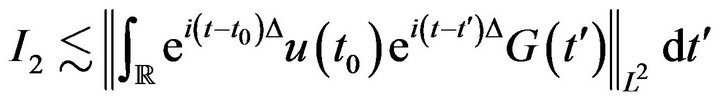
And in this case the lemma follows from the homogeneous estimate proved above. Finally, again by Minkowski’s inequality we have
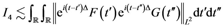
And the proof follows by inserting in the integral the homogeneous estimate above. 
Lemma.4.4. Let  is nearly periodic modulo G. Then there exist functions
 ,
,  and
and , and for every
  there exists
  such that we have the spatial concentration estimate,
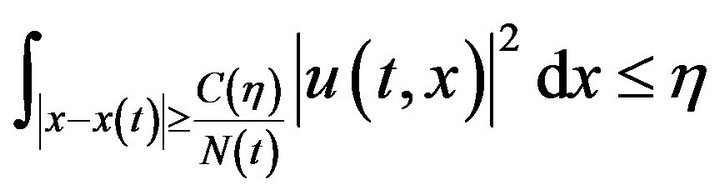 (4.3)
(4.3)
And hesitancy concentration estimate,
 (4.4)
(4.4)
For all 
Remark 4.5. Informally, this lemma confirms that the mass  is spatially concentrated in the ball
 And is hesitancy concentrated in the ball
 .
.
Note that we have presently no control about how ,
,  ,
,  vary in time; (for more see [14- 17]).
Proof: By hypothesis,  lay in GI for some compact subset I in
 . For every
 , compactness argument shows that there exists
 , (depending on) such that

And hesitancy concentration estimate

 For all
 . By inspecting what the symmetry group G does to the spatial and hesitancy distribution of the mass of a function, then the claim follows.
Corollary 4.6. Fix  and d, and assume that m0 is finite. Then there exists a maximal-lifespan solution
  of mass precisely m0 which blows up both forward and backward in time, and functions,
  ,
,  and
and , with property
 , for every
  (depending on
 , d, m0) such that we have the concentration estimates (4.3), (4.4) For all